Filtering with Inverted Indexes

Database queries are all about filtering. Whether you’re finding rows with a particular name, within a price-range, or those created within a time-window. Trouble, however, ensues for most databases when you have many filters and none of them narrow down the results much.

This problem of filtering on many attributes efficiently has haunted me since Problem 3, and again in Problem 9. Queries that mass-filter are conceptually common in commerce merchandising/collections/discovery/discounts where you expect to narrow down products by many attributes. Devilish queries of the type below might be used to create a “Blue Training Sneaker Summer Mega-Sale” collection. The merchant might have tens of millions of products, and each attribute might be on millions of products. In SQL, it might look something like the following:

SELECT id
FROM products
WHERE color=blue AND type=sneaker AND activity=training 
  AND season=summer AND inventory > 0 AND price <= 200 AND price >= 100 

These are especially challenging when you expect the database to return a result in a time-frame that’s suitable for a web request (sub 10 ms). Unfortunately, classic relational databases are typically not suited for serving these types of queries efficiently on their B-Tree based indexes for a few reasons. The two arguments that top the list for me:

1. The data doesn’t conform to a strict schema. A product might have 100s to 1000s of attributes we need to efficiently filter against. This might mean having extremely wide rows, with 100s of indexes, which leads to a number of other issues.
2. Databases struggle to merge multiple indexes.
   1. Index merges not going to get you < 10 ms response, and creating composite indexes are impractical if you are filtering by 10s to 100s of rules. I wrote a separate post about that.
   2. While MySQL/Postgres can filter by price and then type to serve a query, it can’t filter efficiently by scanning and cross-referencing multiple indexes simultaneously (this requires Zig-Zag joins, see here for more context).

Using B-Trees for mass-filtering deserves deeper thought and napkin math (these two problems don’t seem impossible to solve), and given how much this problem troubles me, I might follow up with more detail on this in another issue. It’s also worth noting that Posgres and MySQL both implement inverted indexes, so those could be used instead of the implementation below.

But in this issue we will investigate the inverted index as a possible data-structure for serving many-filter queries efficiently. The inverted index (explained below) is the data-structure that powers search. We will be using Lucene, which is the most popular open-source implementation of the inverted index. It’s what powers ElasticSearch and Solr, the two most popular open-source search engines. You can think of Lucene as the RocksDB/InnoDB of search. Lucene is written in Java.

Why would we want to use a search engine to filter data? Because search as a problem is a superset of our filtering problem. Search is fundamentally about turning a language query blue summer sneakers into a series of filtering operations: intersect products that match blue, summer, and sneaker. Search has a language component, e.g. turning sneakers into sneaker, but the filtering problem is the same. If search is fundamentally language + filtering, perhaps we can use just the filtering bit? Search is typically not implemented on top of B-Tree indexes (what classic databases use), but use an inverted index. Perhaps that can resolve problem (1) and (2) above?

The inverted index is best illustrated through a simple drawing:

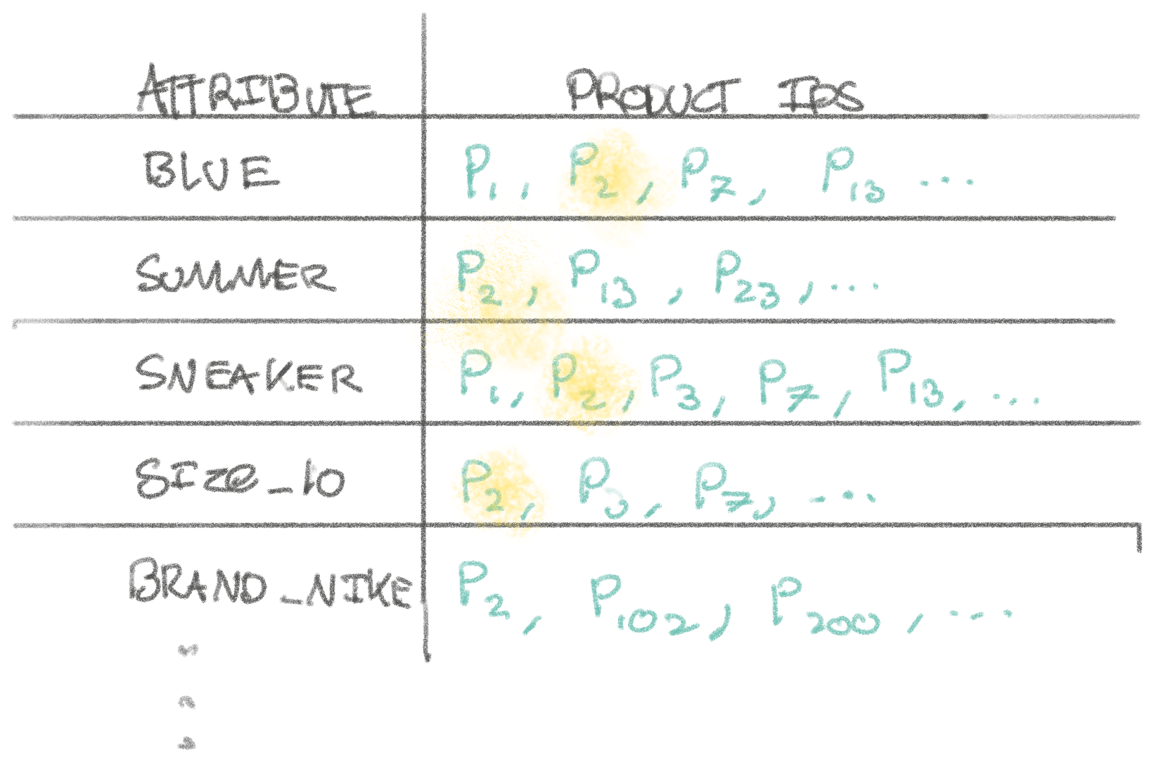
In our inverted index, each attribute (color, type, activity, ..) maps to a list of product ids that have that attribute. We can create a filter for blue, summer, and sneakers by finding the intersection of product ids that match blue, summer, and sneakers (ids that are present for all terms).

Let’s say we have 10 million products, and we are filtering by 3 attributes which each have 1.2 million products in each. What can we expect the query time to be?

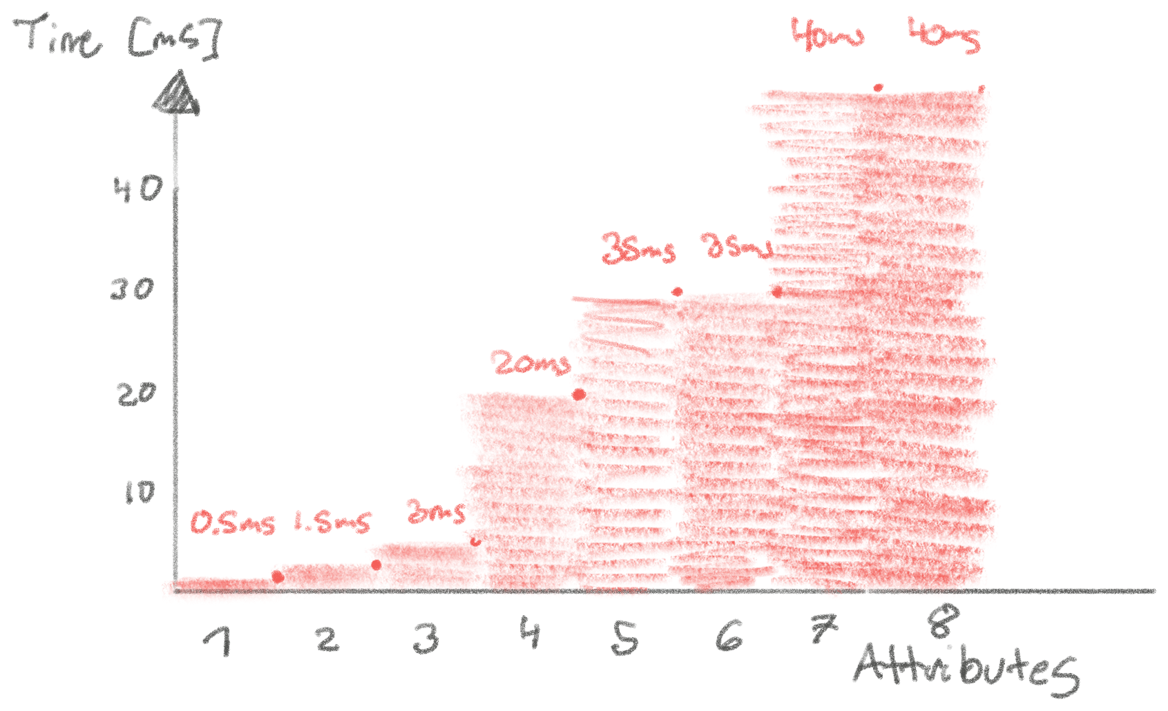
Let’s assume the product ids are stored each as an uncompressed 64 bit integer in memory. We’d expect each attribute to be 1.2 million * 64 bit ~= 10mb, or 10 * 3 = 30mb total. In this case, we assume the intersection algorithm to be efficient and roughly read all the data once (in reality, there’s a lot of smart skipping involved, but this is napkin math. We won’t go into details on how to efficiently merge two sets). We can read memory at a rate of 1 Mb/100 us (from SSD is only twice as slow for sequential reads), so serving the query would take ~0.1 ms * 30 = 3ms. I implemented this in Lucene, and this napkin math lines up well with reality. In my implementation, this takes ~5-3ms! That’s great news for solving the filtering problem with an inverted index. That’s fairly fast.

Now, does this scale linearly? Including more attributes will mean scanning more memory. E.g. 8 attributes we’d expect to scan ~10mb * 8 = 80mb of memory, which should take ~0.1ms * 80 = 8ms. However, in reality this takes 30-60ms. This approaches our napkin math being an order of magnitude off. Most likely this is when we have exhausted the CPU L3 cache, and have to cycle more into main memory. We hit a similar boundary from 3 to 4 attributes. It might also suggest there’s room for optimization in Lucene.

Another interesting to note is that if we look at the inverted index file for our problem, it’s roughly ~261mb. Won’t bore you with the calculation here, but given the implementation this means that we can estimate that each product id takes up ~6.3 bits. This is much smaller than the 64 bits per product id we estimated. The JVM overhead, however, likely makes up for it. Additionally, in Lucene doesn’t just store the product ids, but also various other meta-data along with the product ids.

Based on this, it’s looking feasible to use Lucene for mass filtering! While we don’t have an estimate from SQL to measure against yet (and won’t have in this issue), I can assure you this is faster than we’d get with something naive.

But why is it feasible even if 4 attributes takes ~20ms (as we can see on the diagram)? Because that’s acceptable-ish performance in a worst-worst case scenario. In most cases when you’re filtering, you will have multiple attributes that will be able to significantly narrow the search space. Since we aren’t that close to the lower-bound of performance (what our napkin math tells us), it suggests we might not be constrained by memory bandwidth, but by computation. This suggests that threaded execution could speed it up. And sure enough, it does. With 8 threads in the read thread pool for Lucene, we can serve the query for 4 attributes in ~6ms! That’s faster than our 8ms lower-bound. The reason for this is that Lucene has optimizations built in to skip over potentially large blocks of product ids when intersecting, meaning we don’t have to read all the product ids in the inverted index.

In reality, to go further, we’d want to do more napkin math, but this is showing a lot of promise! Besides more calculations, we’ve left out two big pieces here: sorting and indexing numbers. If there’s interest, I might follow up with that another time. But this is plenty for one issue!

You might also like...

• MySQL transactions per second vs fsyncs per second
• Using checksums to verify syncing 100M database records
• Shitlist Driven Development
• Neural Network From Scratch
• Inverted Index Performance and Merkle Tree Syncronization