SELECT count(*) /* matches ~100 rows out of 10M */
FROM table
WHERE int1000 = 1 AND int100 = 1
/* int100 rows are 0..99 and int1000 0...9999 */
create table test_table (
id bigint primary key not null,
text1 text not null, /* 1 KiB of random data */
text2 text not null, /* 255 bytes of random data */
/* cardinality columns */
int1000 bigint not null, /* ranges 0..999, cardinality: 1000 */
int100 bigint not null, /* 0..99, card: 100 */
int10 bigint not null, /* 0..10, card: 10 */
);
/* no indexes yet, we create those in the sections below */
We can create a composite index on (int1000, int100)
, or we could have two
individual indexes on (int1000)
and (int100)
, relying on the database to
leverage both indexes.
Having a composite index is faster, but how much faster than the two individual indexes? Let’s do the napkin math, and then test it in PostgreSQL and MySQL.
We’ll start with the napkin math, and then verify it against Postgres and MySQL.
The ideal index for this count(*)
is:
CREATE INDEX ON table (int1000, int100)
It allows the entire count to be performed on this one index.
WHERE int1000 = 1 AND int100 = 1
matches ~100 records of the 10M total for the
table. 1 The database would do a quick search in the index tree to the leaf in the
index where both columns are 1
, and then scan forward until the condition no
longer holds.
For these 64-bit index entries we’d expect to have to scan only the ~100 entries that match, which is a negligible ~2 KiB. According to the napkin reference, we can read from memory, so this will take absolutely no time. With the query overhead, navigating the index tree, and everything else, it theoretically shouldn’t take a database more than a couple on the composite index to satisfy this query. 2
But a database can also do an index merge of two separate indexes:
CREATE INDEX ON table (int1000)
CREATE INDEX ON table (int100)
But how does a database utilize two indexes? And how expensive might this merge be?
How indexes are intersected depends on the database! There are many ways of finding the intersection of two unordered lists: hashing, sorting, sets, KD-trees, bitmap, …
MySQL does what it calls an index merge intersection, I haven’t consulted
the source, but most likely it’s sorting. Postgres does index intersection by
generating a bitmap after scanning each index, and then AND
ing them
together.
int100 = 1
returns about rows, which is
about ~1.5 MiB to scan. int1000 = 1
matches only ~10,000 rows, so in total
we’re reading about 200 μs worth of memory from both indexes.
After we have the matches from the index, we need to intersect them. In this case, for simplicity of the napkin math, let’s assume we sort the matches from both indexes and then intersect from there.
We can sort in . So it would take us ~10ms total to sort it, iterate through both sorted lists for a negligible of memory reading, write the intersection to memory for another , and then we’ve got the interesection, i.e. rows that match both conditions.
Thus our napkin math indicates that for our two separate indexes we’d expect the
query to take . The sorting is sensitive to the index size which
is fairly approximate, so give it a low multiplier to land at, ~10-30ms
.
As we’ve seen, intersection bears a meaningful cost and on paper we expect it to be roughly an order of magnitude slower than composite indexes. However, 10ms is still sensible for most situations, and depending on the situation it might be nice to not have a more specialized composite index for the query! For example, if you are often joining between a subset of 10s of columns.
Now that we’ve set our expectations from first principles about composite indexes versus merging multiple indexes, let’s see how Postgres and MySQL fare in real-life.
Both MySQL and Postgres perform index-only scans after we create the index:
/* 10M rows total, int1000 = 1 matches ~10K, int100 matches ~100K */
CREATE INDEX ON table (int1000, int100)
EXPLAIN ANALYZE SELECT count(*) FROM table WHERE int1000 = 1 AND int100 = 1
/* postgres, index is ~70 MiB */
Aggregate (cost=6.53..6.54 rows=1 width=8) (actual time=0.919..0.919 rows=1 loops=1)
-> Index Only Scan using compound_idx on test_table (cost=0.43..6.29 rows=93 width=0) (actual time=0.130..0.909 rows=109 loops=1)
Index Cond: ((int1000 = 1) AND (int100 = 1))
Heap Fetches: 0
/* mysql, index is ~350 MiB */
-> Aggregate: count(0) (cost=18.45 rows=1) (actual time=0.181..0.181 rows=1 loops=1)
-> Covering index lookup on test_table using compound_idx (int1000=1, int100=1) (cost=9.85 rows=86) (actual time=0.129..0.151 rows=86 loops=1)
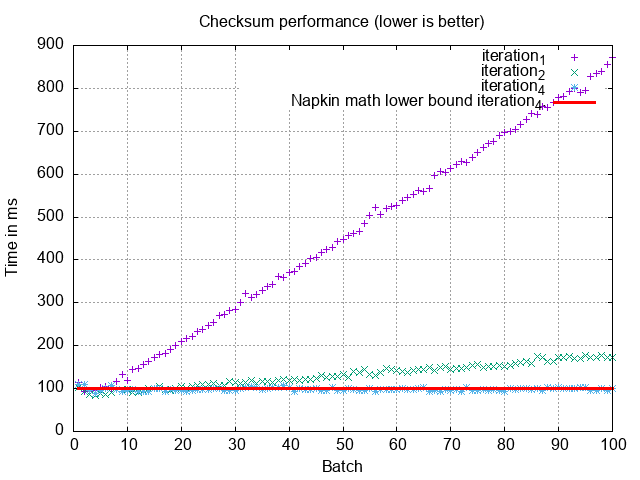
They each take about ~3-5ms when the index is cached. It is a bit slower than the ~1ms we expected from the napkin math, but in our experience working with napkin math on database, tracks within an order of magnitude to seem acceptable. We attribute this to overhead of walking through the index. 3
When we execute the query in MySQL it takes ~30-40ms, which tracks well the upper end of our napkin math. That means our first principle understanding likely lines up with reality!
Let’s confirm it’s doing what we expect by looking at the query plan:
/* 10M rows total, int1000 = 1 matches ~10K, int100 matches ~100K */
EXPLAIN ANALYZE SELECT count(*) FROM table WHERE int1000 = 1 AND int100 = 1
/* mysql, each index is ~240 MiB */
-> Aggregate: count(0) (cost=510.64 rows=1) (actual time=31.908..31.909 rows=1 loops=1)
-> Filter: ((test_table.int100 = 1) and (test_table.int1000 = 1)) (cost=469.74 rows=409) (actual time=5.471..31.858 rows=86 loops=1)
-> Intersect rows sorted by row ID (cost=469.74 rows=410) (actual time=5.464..31.825 rows=86 loops=1)
-> Index range scan on test_table using int1000 over (int1000 = 1) (cost=37.05 rows=18508) (actual time=0.271..2.544 rows=9978 loops=1)
-> Index range scan on test_table using int100 over (int100 = 1) (cost=391.79 rows=202002) (actual time=0.324..24.405 rows=99814 loops=1)
/* ~30 ms */
MySQL’s query plan tells us it’s doing exactly as we expected: get the
matching entries from each index, intersecting them and performing the count on
the intersection. Running EXPLAIN
without analyze I could confirm that it’s
serving everything from the index and never going to seek the full row.
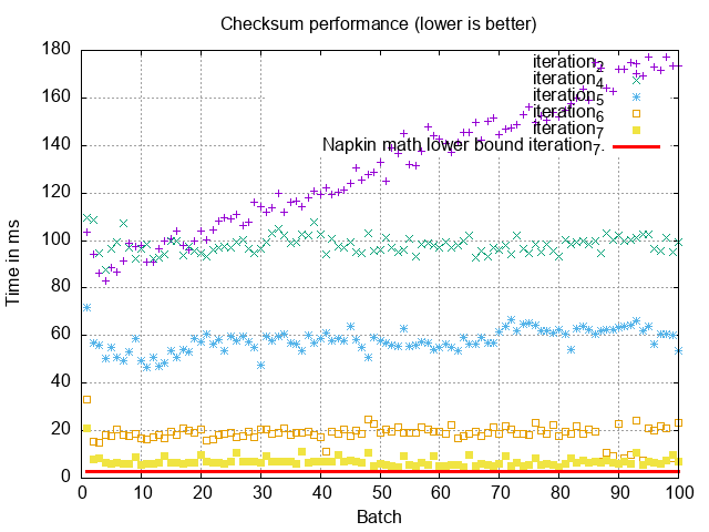
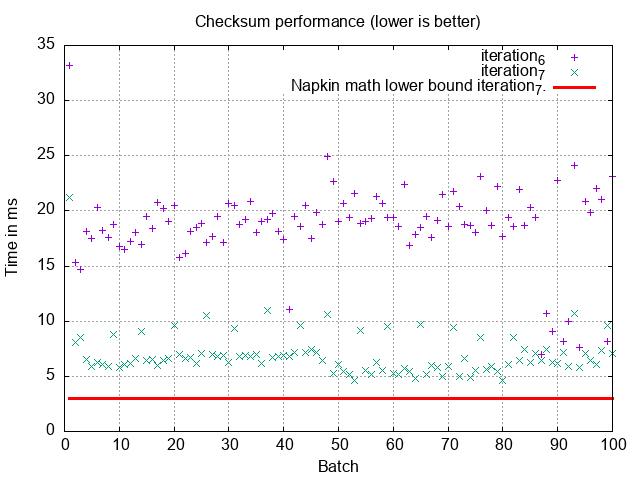
Postgres is also within an order of magnitude of our napkin math, but it’s on the higher range with more variance, in general performing worse than MySQL. Is its bitmap-based intersection just slower on this query? Or is it doing something completely different than MySQL?
Let’s look at the query plan using the same query as we used from MySQL:
/* 10M rows total, int1000 = 1 matches ~10K, int100 matches ~100K */
EXPLAIN ANALYZE SELECT count(*) FROM table WHERE int1000 = 1 AND int100 = 1
/* postgres, each index is ~70 MiB */
Aggregate (cost=1536.79..1536.80 rows=1 width=8) (actual time=29.675..29.677 rows=1 loops=1)
-> Bitmap Heap Scan on test_table (cost=1157.28..1536.55 rows=95 width=0) (actual time=27.567..29.663 rows=109 loops=1)
Recheck Cond: ((int1000 = 1) AND (int100 = 1))
Heap Blocks: exact=109
-> BitmapAnd (cost=1157.28..1157.28 rows=95 width=0) (actual time=27.209..27.210 rows=0 loops=1)
-> Bitmap Index Scan on int1000_idx (cost=0.00..111.05 rows=9948 width=0) (actual time=2.994..2.995 rows=10063 loops=1)
Index Cond: (int1000 = 1)
-> Bitmap Index Scan on int100_idx (cost=0.00..1045.94 rows=95667 width=0) (actual time=23.757..23.757 rows=100038 loops=1)
Index Cond: (int100 = 1)
Planning Time: 0.138 ms
/* ~30-90ms */
The query plan confirms that it’s using the bitmap intersection strategy for intersecting the two indexes. But that’s not what’s causing the performance difference.
While MySQL services the entire aggregate (count(*)
) from the index, Postgres
actually goes to the heap to get every row. The heap contains the entire
row, which is upwards of 1 KiB. This is expensive, and when the heap cache isn’t
warm, the query takes almost 100ms! 4
As we can tell from the query plan, it seems that Postgres is unable to do index-only scans in conjunction with index intersection. Maybe in a future Postgres version they will support this; I don’t see any fundamental reason why they couldn’t!
Going to the heap doesn’t have a huge impact when we’re only going to the heap
for 100 records, especially when it’s cached. However, if we change the
condition to WHERE int10 = 1 and int100 = 1
, for a total of 10,000 matches,
then this query takes 7s on Postgres, versus 200ms in MySQL where the index-only
scan is alive and kicking!
So MySQL is superior on index merges where there is an opportunity to service the entire query from the index. It is worth pointing out though that Postgres’ lower-bound when everything is cached is lower for this particular intersection size, likely its bitmap-based intersection is faster.
Postgres and MySQL do have roughly equivalent performance on index-only scans
though. For example, if we do int10 = 1
Postgres will do its own index-only
scan because only one index is involved.
The first time I ran Postgres for this index-only scan it was taking over a
second, I had to run VACUUM
for the performance to match! Index-only scans
require frequent VACUUM
on the table to avoid going to the heap to fetch the
entire row in Postgres.
VACUUM
helps because Postgres has to visit the heap for any records that have
been touched since the last VACUUM
, due to its MVCC implementation. In my
experience, this can have serious consequences in production for index-only
scans if you have an update-heavy table where VACUUM
is expensive.
Index merges are ~10x slower than composite indexes because the ad-hoc intersection isn’t a very fast operation. It requires e.g. sorting of the output of each index scan to resolve. Indexes could be optimized further for intersection, but this would likely have other ramifications for steady-state load.
If you’re wondering if you need to add a composite index, or can get away with creating to single indexes and rely on the database to use both indexes — then the rule of thumb we establish is that an index merge will be ~10x slower than the composite index. However, we’re still talking less than 100ms in most cases, as long as you’re operating on 100s of rows (which in a relational, operational database, hopefully you mostly are).
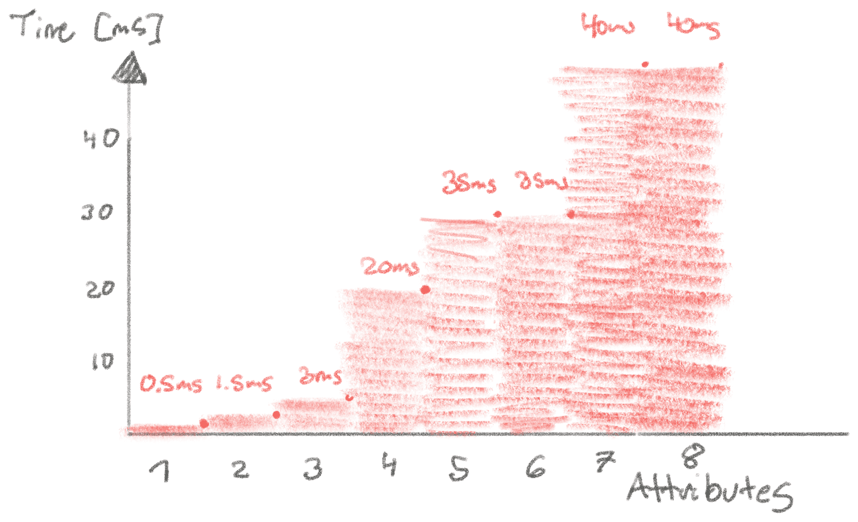
The gap in performance will widen when intersecting more than two columns, and with a larger intersection size—I had to limit the scope of this article somewhere. Roughly an order of magnitude seems like a reasonable assumption, with ~100 rows matching many real-life query averages.
If you are using Postgres, be careful relying on index merging! Postgres doesn’t
do index-only scans after an index merge, requiring going to the heap for
potentially 100,000s of records for a count(*)
. If you’re only returning 10s
to 100s of rows, that’s usually fine.
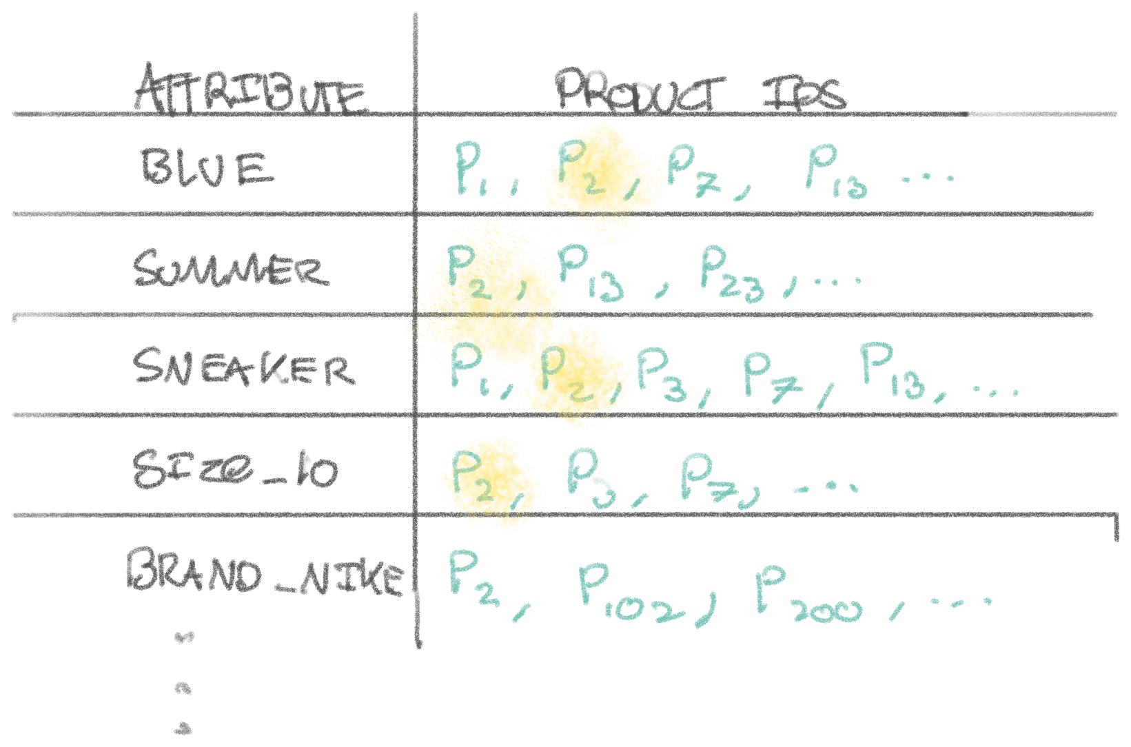
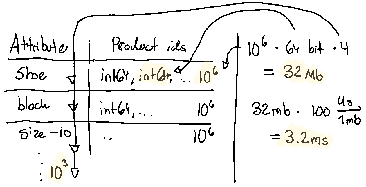
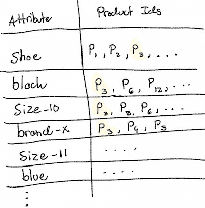
Another second-order take-away: If you’re in a situation where you have 10s of columns filtering in all kinds of combinations, with queries like this:
SELECT id
FROM products
WHERE color=blue AND type=sneaker AND activity=training
AND season=summer AND inventory > 0 AND price <= 200 AND price >= 100
/* and potentially many, many more rules */
Then you’re in a bit more of a pickle with Postgres/MySQL. It would require a combinatoric explosion of composite indexes to support this use-case well, which would be critical for sub 10ms performance required for fast websites. This is simply unpractical.
Unfortunately, for sub 10ms response times, we also can’t rely on index merges being that fast, because of the ad-hoc interesection. I wrote an article about solving the problem of queries that have lots of conditions with Lucene, which is very good at doing lots of intersections. It would be interesting to try this with GIN-indexes (inverted index, similar to what Lucene does) in Postgres as a comparison. Bloom-indexes may also be suited for this. Columnar database might also be better at this, but I haven’t looked at that in-depth yet.
The testing is done on a table generated by this simple script. ↩
There’s a extra overhead searching the index B-tree to the relevant range, and the reads aren’t entirely sequential in the B-tree. Additionally, we’re assuming the index is in memory. That’s a reasonable assumption given the tiny size of the index. From SSD should only be 2x slower since it’s mostly sequential-ish access once the relevant first leaf has been found. Each index entry struct is also bigger than two 64 bit integers, e.g. the heap location in Postgres or the primary key in MySQL. Either way, napkin math of a few hundred microseconds still seems fair! ↩
Looking at the real index sizes, the compound index is ~70 MiB in Postgres, and 350 MiB in MySQL. We’d expect the entire index of ~3 64 bit integers (the third being the location on the heap) to be ~230 MiB for 10M rows. fabien2k on HN pointed out that Postgres does de-duplication, which is likely how it achieves its lower index size. MySQL has some overhead, which is reasonable for a structure of this size. They both perform about equally though on this, but a smaller index size at the same performance is superior as it takes less cache space. ↩
In the first edition of this article, Postgres was going to the heap 100s
of times, instead of just for 109 times for the 109 matching rows. It turns
out it’s because the bitmaps and the intersection was exceeding the
work_mem=4MB
default setting. This causes Postgres to use a lossy bitmap
intersection with the just the heap page rather than exact row location. Read
more here. Thanks to /u/therealgaxbo and /u/trulus on Reddit for
pointing this out. Either way, Postgres is still not performing an
index-only scan, requiring 109 random disk seeks on a cold cache taking ~90ms. ↩
Causal is a spreadsheet built for the 21st century to help people work better
with numbers. Behind Causal’s innocent web UI is a complex calculation engine —
an interpreter that executes formulas on an in-memory, multidimensional
database. The engine sends the result from evaluating expressions like Price * Units
to the browser. The engine calculates the result for each dimension such
as time, product name, country e.g. what the revenue was for a single product,
during February ‘22, in Australia.
In the early days of Causal, the calculation engine ran in Javascript in the browser, but that only scaled to 10,000s of cells. So we moved the calculation engine out of the browser to a Node.js service, getting us to acceptable performance for low 100,000s of cells. In its latest and current iteration, we moved the calculation engine to Go, getting us to 1,000,000s of cells.
But every time we scale up by an order of magnitude, our customers find new use-cases that require yet another order of magnitude more cells!
With no more “cheap tricks” of switching the run-time again, how can we scale the calculation engine 100x, from millions to billions of cells?
In summary: by moving from maps to arrays. 😅 That may seem like an awfully pedestrian observation, but it certainly wasn’t obvious to us at the outset that this was the crux of the problem!
We want to take you along our little journey of what to do once you’ve reached a dead-end with the profiler. Instead, we’ll be approaching the problem from first principles with back-of-the envelope calculations and writing simple programs to get a feel for the performance of various data structures. Causal isn’t quite at billions of cells yet, but we’re rapidly making our way there!
What does it look like to reach a dead-end with a profiler? When you run a profiler for the first time, you’ll often get something useful: your program’s spending 20% of time in an auxiliary function log_and_send_metrics()
that you know reasonably shouldn’t take 20% of time.
You peek at the function, see that it’s doing a ridiculous amount of string allocations, UDP-jiggling, and blocking the computing thread… You play this fun and rewarding profile whack-a-mole for a while, getting big and small increments here and there.
But at some point, your profile starts to look a bit like the above: There’s no longer anything that stands out to you as grossly against what’s reasonable. No longer any pesky log_and_send_metrics()
eating double-digit percentages of your precious runtime.
The constraints move to your own calibration of what % is reasonable in the profile: It’s spending time in the GC, time allocating objects, a bit of time accessing hash maps, … Isn’t that all reasonable? How can we possibly know whether 5.3% of time scanning objects for the GC is reasonable? Even if we did optimize our memory allocations to get that number to 3%, that’s a puny incremental gain… It’s not going to get us to billions of cells! Should we switch to a non-GC’ed language? Rust?! At a certain point, you’ll go mad trying to turn a profile into a performance roadmap.
When analyzing a system top-down with a profiler, it’s easy to miss the forest for the trees. It helps to take a step back, and analyze the problem from first principles.
We sat down and thought about fundamentally, what is a calculation engine? With some back-of-the-envelope calculations, what’s the upper bookend of how many cells we could reasonably expect the Calculation engine to support?
In my experience, first-principle thinking is required to break out of iterative improvement and make order of magnitude improvements. A profiler can’t be your only performance tool.
To understand, we have to explain two concepts from Causal that help keep your spreadsheet organized: dimensions and variables.
We might have a variable “Sales’” that is broken down by the dimensions “Product” and “Country”. To appreciate how easy it is to build a giant model, if we have 100s of months, 10,000s of products, 10s of countries, and 100 variables we’ve already created a model with 1B+ cells. In Causal “Sales” looks like this:
In a first iteration we might represent Sales
and its cells with a map. This seems innocent enough. Especially when you’re coming from an original implementation in Javascript, hastily ported to Go. As we’ll learn in this blog post, there are several performance problems with this data structure, but we’ll take it step by step:
sales := make(map[int]*Cell)
The integer index would be the _dimension index _to reference a specific cell. It is the index representing the specific dimension combination we’re interested in. For example, for Sales[Toy-A][Canada]
the index would be 0 because Toy-A is the 0th Product Name
and Canada is the 0th Country
. For Sales[Toy-A][United Kingdom]
it would be 1 (0th Toy, 1st Country), for Sales[Toy-C][India]
it would be 3 * 3 = 9.
An ostensible benefit of the map structure is that if a lot of cells are 0, then we don’t have to store those cells at all. In other words, this data structure seems useful for sparse models.
But to make the spreadsheet come alive, we to calculate formulas such as Net Profit = Sales * Profit
. This simple equation shows the power of Causal’s dimensional calculations, as this will calculate each cell’s unique net profit!
Now that we have a simple mental model of how Causal’s calculation engine works, we can start reasoning about its performance from first principles.
If we multiply two variables of 1B cells of 64 bit floating points each (~8 GiB memory) into a third variable, then we have to traverse at least ~24 GiB of memory. If we naively assume this is sequential access (which hashmap access isn’t) and we have SIMD and multi-threading, we can process that memory at a rate of 30ms / 1 GiB, or ~700ms total (and half that time if we were willing to drop to 32-bit floating points and forgo some precision!).
So from first-principles, it seems possible to do calculations of billions of
cells in less than a second. Of course, there’s far more complexity below the
surface as we execute the many types of formulas, and computations on
dimensions. But there’s reason for optimism! We will carry through this example
of multiplying variables for Net Profit
as it serves as a good proxy for the
performance we can expect on large models, where typically you’ll have fewer,
smaller variables.
In the remainder of this post, we will try to close the gap between smaller Go prototypes and the napkin math. That should serve as evidence of what performance work to focus on in the 30,000+ line of code engine.
map[int]*Cell
, 30m cells in ~6sIn Causal’s calculation engine each Cell
in the map was initially ~88 bytes to store various information about the cell such as the formula, dependencies, and other references. We start our investigation by implementing this basic data-structure in Go.
With 10M cell variables, for a total of 30M cells, it takes almost 6s to compute the Net Profit = Sales * Profit
calculation. These numbers from our prototype doesn’t include all the other overhead that naturally accompanies running in a larger code-base, that’s far more feature-complete. In the real engine, this takes a few times longer.
We want to be able to do billions in seconds with plenty of wiggle-room for necessary overhead, so 10s of millions in seconds won’t fly. We have to do better. We know from our napkin math, that we should be able to.
$ go build main.go && hyperfine ./main
Benchmark 1: ./napkin
Time (mean ± σ): 5.828 s ± 0.032 s [User: 10.543 s, System: 0.984 s]
Range (min ... max): 5.791 s ... 5.881 s 10 runs
package main
import (
"math/rand"
)
type Cell88 struct {
padding [80]byte // just to simulate what would be real stuff
value float64
}
func main() {
pointerMapIntegerIndex(10_000_000) // 3 variables = 30M total
}
func pointerMapIntegerIndex(nCells int) {
one := make(map[int]*Cell88, nCells)
two := make(map[int]*Cell88, nCells)
res := make(map[int]*Cell88, nCells)
rand := rand.New(rand.NewSource(0xCA0541))
for i := 0; i < nCells; i++ {
one[i] = &Cell88{value: rand.Float64()}
two[i] = &Cell88{value: rand.Float64()}
}
for i := 0; i < nCells; i++ {
res[i] = &Cell88{value: one[i].value * two[i].value}
}
}
[]Cell
, 30m cells in ~400msIn our napkin math, we assumed sequential memory access. But hashmaps don’t do sequential memory access. Perhaps this is a far larger offender than our profile above might seemingly suggest?
Well, how do hashmaps work? You hash a key to find the bucket that this key/value pair is stored in. In that bucket, you insert the key and value. When the average size of the buckets grows to around ~6.5 entries, the number of buckets will double and all the entries will get re-shuffled (fairly expensive, and a good size to pre-size your maps). The re-sizing occurs to about equality on a lot of keys in ever-increasing buckets.
Let’s think about the performance implications of this from the ground up. Every time we look up a cell from its integer index, the operations we have to perform (and their performance, according to the napkin math reference):
Most of this goes out the wash, by far the most expensive are these random memory reads that the map entails. Let’s say ~100ns per look-up, and we have ~30M of them, that’s ~3 seconds in hash lookups alone. That lines up with the performance we’re seeing. Fundamentally, it really seems like trouble to get to billions of cells with a map.
There’s another problem with our data structure in addition to all the pointer-chasing leading to slow random memory reads: the size of the cell. Each cell is 88 bytes. When a CPU reads memory, it fetches one cache line of 64 bytes at a time. In this case, the entire 88 byte cell doesn’t fit in a single cache line. 88 bytes spans two cache lines, with 128 - 88 = 40 bytes of wasteful fetching of our precious memory bottleneck!
If those 40 bytes belonged to the next cell, that’s not a big deal, since we’re about to use them anyway. However, in this random-memory-read heavy world of using a hashmap that stores pointers, we can’t trust that cells will be adjacent. This is enormously wasteful for our precious memory bandwidth.
In the napkin math reference, random memory reads are ~50x slower than sequential access. A huge reason for this is that the CPU’s memory prefetcher cannot predict memory access. Accessing memory is one of the slowest things a CPU does, and if it can’t preload cache lines, we’re spending _a lot _of time stalled on memory.
Could we give up the map? We mentioned earlier that a nice property of the map is that it allows us to build sparse models with lots of empty cells. For example, cohort models tend to have half of their cells empty. But perhaps half of the cells being empty is not quite enough to qualify as ‘sparse’?
We could consider mapping the index for the cells into a large, pre-allocated array. Then cell access would be just a single random-read of 50ns! In fact, it’s even better than that: In this particular Net Profit
, all the memory access is sequential. This means that the CPU can be smart and prefetch memory because it can reasonably predict what we’ll access next. For a single thread, we know we can do about 1 GiB/100ms. This is about , so it should take somewhere in the ballpark of 250-300ms. Consider also that the allocations themselves on the first few lines take a bit of time.
func arrayCellValues(nCells int) {
one := make([]Cell88, nCells)
two := make([]Cell88, nCells)
res := make([]Cell88, nCells)
rand := rand.New(rand.NewSource(0xCA0541))
for i := 0; i < nCells; i++ {
one[i].value = rand.Float64()
two[i].value = rand.Float64()
}
for i := 0; i < nCells; i++ {
res[i].value = one[i].value * two[i].value
}
}
napkin:go2 $ go build main.go && hyperfine ./main
Benchmark 1: ./main
Time (mean ± σ): 346.4 ms ± 21.1 ms [User: 177.7 ms, System: 171.1 ms]
Range (min ... max): 332.5 ms ... 404.4 ms 10 runs
That’s great! And it tracks our expectations from our napkin math well (the extra overhead is partially from the random number generator).
Generally, we expect threading to speed things up substantially as we’re able to utilize more cores. However, in this case, we’re memory bound, not computationally bound. We’re just doing simple calculations between the cells, which is generally the case in real Causal models. Multiplying numbers takes single-digit cycles, fetching memory takes double to triple-digit number of cycles. Compute bound workloads scale well with cores. Memory bound workloads act differently when scaled up.
If we look at raw memory bandwidth numbers in the napkin math reference, a 3x speed-up in a memory-bound workload seems to be our ceiling. In other words, if you’re memory bound, you only need about ~3-4 cores to exhaust memory bandwidth. More won’t help much. But they do help, because a single thread cannot exhaust memory bandwidth on most CPUs.
When implemented however, we only get a 0.6x speedup (400ms → 250ms), and not a 3x speed-up (130ms)? I am frankly not sure how to explain this ~120ms gap. If anyone has a theory, we’d love to hear it!
Either way, we definitely seem to be memory bound now. Then there’s only two ways forward: (1) Get more memory bandwidth on a different machine, or (2) Reduce the amount of memory we’re using. Let’s try to find some more brrr with (2).
If we were able to cut the cell size 3x from 88 bytes to 32 bytes, we’d expect the performance to roughly 3x as well! In our simulation tool, we’ll reduce the size of the cell:
type Cell32 struct {
padding [24]byte
value float64
}
Indeed, with the threading on top, this gets us to ~70ms which is just around a 3x improvement!
In fact, what is even in that cell struct? The cell stores things like formulas, but for many cells, we don’t actually need the formula stored with the cell. For most cells in Causal, the formula is the same as the previous cell. I won’t show the original struct, because it’s confusing, but there are other pointers, e.g. to the parent variable. By more carefully writing the calculation engine’s interpreter to keep track of the context, we should be able to remove various pointers to e.g. the parent variable. Often, structs get expanded with cruft as a quick way to break through some logic barrier, rather than carefully executing the surrounding context to provide this information on the stack.
As a general pattern, we can reduce the size of the cell by switching from an array of structs design to a struct of arrays design, in other words, if we’re in a cell with index 328, and need the formula for the cell, we could look up index 328 in a formula array. These are called parallel arrays. Even if we access a different formula for every single cell the CPU is smart enough to detect that it’s another sequential access. This is generally much faster than using pointers.
None of this is particularly hard to do, but it wasn’t until now that we realized how paramount this was to the engine’s performance! Unfortunately, the profiler isn’t yet helpful enough to tell you that reducing the size of a struct below that 64-byte threshold can lead to non-linear performance increases. You need to know to use tools like pahole(1)
for that.
[]float64
w/ Parallel Arrays, 20msIf we want to find the absolute speed-limit for Causal’s performance then, we’d want to imagine that the Cell is just:
type Cell8 struct {
value float64
}
That’s a total memory usage of which we can read at 35 μs/MiB in a threaded program, so ~8ms. We won’t get much faster than this, since we also inevitably have to spend time allocating the memory.
When implemented, the raw floats take ~20ms (consider that we have to allocate the memory too) for our 30M cells.
Let’s scale it up. For 1B cells, this takes ~3.5s. That’s pretty good! Especially considering that the Calculation engine already has a lot of caching already to ensure we don’t have to re-evaluate every cell in the sheet. But, we want to make sure that the worst-case of evaluating the entire sheet performs well, and we have some space for inevitable overhead.
Our initial napkin math suggested we could get to ~700ms for 3B cells, so there’s a bit of a gap. We get to ~2.4s for 1B cells by moving allocations into the threads that actually need them, closing the gap further would take some more investigation. However, localizing allocations start to get into a territory of what would be quite hard to implement generically in reality—so we’ll stop around here until we have the luxury of this problem being the bottleneck. Plenty of work to make all these transitions in a big, production code-base!
That said, there are lots of optimizations we can do. Go’s compiler currently doesn’t do SIMD, which allows us to get even more memory bandwidth. Another path for optimization that’s common for number-heavy programs is to encode the numbers, e.g. delta-encoding. Because we’re constrained by memory bandwidth more than compute, counter-intuitively, compression can make the program faster. Since the CPU is stalled for tons of cycles while waiting for memory access, we can use these extra cycles to do simple arithmetic to decompress.
Another trend from the AI-community when it comes to number-crunching too is to leverage GPUs. These have enormous memory bandwidth. However, we can create serious bottlenecks when it comes to moving memory back and forth between the CPU and GPU. We’d have to learn what kinds of models would take advantage of this, we have little experience with GPUs as a team—but we may be able to utilize lots of existing ND-array implementations used for training neural nets. This would come with significant complexity—but also serious performance improvements for large models.
Either way there’s plenty of work to get to the faster, simpler design described above in the code-base. This would be further out, but makes us excited about the engineering ahead of us!
Profiling had become a dead-end to make the calculation engine faster, so we needed a different approach. Rethinking the core data structure from first principles, and understanding exactly why each part of the current data structure and access patterns was slow got us out of disappointing, iterative single-digit percentage performance improvements, and unlocked order of magnitude improvements. This way of thinking about designing software is often referred to as data-oriented engineering, and this talk by Andrew Kelly, the author of the Zig compiler, is an excellent primer that was inspirational to the team.
With these results, we were able to build a technical roadmap for incrementally moving the engine towards a more data-oriented design. The reality is _far _more complicated, as the calculation engine is north of 40K lines of code. But this investigation gave us confidence in the effort required to change the core of how the engine works, and the performance improvements that will come over time!
The biggest performance take-aways for us were:
Causal doesn’t smoothly support 1 billion cells yet, but we feel confident in our ability to iterate our way there. Since starting this work, our small team has already improved performance more than 3x on real models. If you’re interested in working on this with Causal, and them get to 10s of billions of cells, you should consider joining the Causal team — email lukas@causal.app!
]]>p50
, p90
, p99
, sum
, avg
†/min
p50
, p90
, p99
%
†/min
p50
, p90
, p99
, sum
, avg
†{error, success, retry}
†p50
, p90
, p99
, count
, by type
†/min
† Metrics where you need the ability to slice by endpoint
or job
,
tenant_id
, app_id
, worker_id
, zone
, hostname
, and queue
(for jobs).
This is paramount to be able to figure out if it’s a single endpoint, tenant, or
app that’s causing problems.
You can likely cobble a workable chunk of this together from your existing service provider and APM. The value is for you to know what metrics to pay attention to, and which key ones you’re missing. The holy grail is one dashboard for web, and one for job. The more incidents you have, the more problematic it becomes that you need to visit a dozen URLs to get the metrics you need.
If you have little of this and need somewhere to start, start with logs. They’re the lowest common denominator, and if you’re productive in a good logging system that will you very far. You can build all these dashboards with logs alone. Jumping into the detailed logs is usually the next step you take during an incident if it’s not immediately clear what to do from the metrics.
Use the canonical log line pattern (see figure below), resist emitting random logs throughout the request as this makes analysis difficult. A canonical log line is a log emitted at the end of the request with everything that happened during the request. This makes querying the logs bliss.
Surprisingly, there aren’t good libraries available for the canonical log line pattern, so I recommend rolling your own. Create a middleware in your job and web stack to emit the log at the end of the request. If you need to accumulate metrics throughout the request for the canonical log line, create a thread-local dictionary for them that you flush in the middleware.
For response time from services, you will need to emit inline logs or metrics. Consider using an OpenTelemetry library so you only need to instrument once and can later add sinks for canonical logs (the sum), metrics, profiling, and traces.
Notably absent here is monitoring a database, which would take its own post.
Hope this helps you step up your monitoring game. If there’s a metric you feel strongly that’s missing, please let me know!
This is one of my favorites. What percentage of threads are
currently busy? If this is >80%
, you will start to see counter-intuitive
queuing theory take hold, yielding strange response time patterns.
It is given as busy_threads / total_threads
. ↩
How long are requests spending in TCP/proxy queues before being
picked up by a thread? Typically you get this by your load-balancer stamping
the request with a X-Request-Start
header, then subtracting that from the
current time in the worker thread. ↩
Same idea as web utilization, but in this case it’s OK for it to be > 80% for periods of time as jobs are by design allowed to be in the queue for a while. The central metric for jobs becomes time in queue. ↩
The central metric for monitoring a job stack is to know how long jobs spend in the queue. That will be what you can use to answer questions such as: Do I need more workers? When will I recover? What’s the experience for my users right now? ↩
How large is your queue right now? It’s especially amazing to be able to slice this by job and queue, but your canonical logs with how much has been enqueued is typically sufficient. ↩
Neural nets are increasingly dominating the field of machine learning / artificial intelligence: the most sophisticated models for computer vision (e.g. CLIP), natural language processing (e.g. GPT-3), translation (e.g. Google Translate), and more are based on neural nets. When these artificial neural nets reach some arbitrary threshold of neurons, we call it deep learning.
A visceral example of Deep Learning’s unreasonable effectiveness comes from this interview with Jeff Dean who leads AI at Google. He explains how 500 lines of Tensorflow outperformed the previous ~500,000 lines of code for Google Translate’s extremely complicated model. Blew my mind. 1
As a software developer with a predominantly web-related skillset of Ruby, databases, enough distributed systems knowledge to know to not get fancy, a bit of hard-earned systems knowledge from debugging incidents, but only high school level math: neural networks mystify me. How do they work? Why are they so good? Why are they so slow? Why are GPUs/TPUs used to speed them up? Why do the biggest models have more neurons than humans, yet still perform worse than the human brain? 2
In true napkin math fashion, the best course of action to answer those questions is by implementing a simple neural net from scratch.
The hardest part of napkin math isn’t the calculation itself: it’s acquiring the conceptual understanding of a system to come up with an equation for its performance. Presenting and testing mental models of common systems is the crux of value from the napkin math series!
The simplest neural net we can draw might look something like this:
[1, 1, 1, 0.2]
. Meaning the first 3 pixels are darkest (1.0) and the last pixel is
lighter (0.2).0.8
.For example for the image = [0.8, 0.7, 1, 1]
we’d expect a value close to 1 (dark!).
In contrast, for = [0.2, 0.5, 0.4, 0.7]
we
expect something closer to 0 than to 1.
Let’s implement a neural network from our simple mental model. The goal of this neural network is to take a grayscale 2x2 image and tell us how “dark” it is where 0 is completely white , and 1 is completely black . We will initialize the hidden layer with some random values at first, in Python:
input_layer = [0.2, 0.5, 0.4, 0.7]
# We randomly initialize the weights (values) for the hidden layer... We will
# need to "train" to make these weights give us the output layers we desire. We
# will cover that shortly!
hidden_layer = [0.98, 0.4, 0.86, -0.08]
output_neuron = 0
# This is really matrix multiplication. We explicitly _do not_ use a
# matrix/tensor, because they add overhead to understanding what happens here
# unless you work with them every day--which you probably don't. More on using
# matrices later.
for index, input_neuron in enumerate(input_layer):
output_neuron += input_neuron * hidden_layer[index]
print(output_neuron)
# => 0.68
Our neural network is giving us model() = 0.7
which is closer to ‘dark’ (1.0) than ‘light’ (0.0). When looking
at this rectangle as a human, we judge it to be more bright than dark, so we
were expecting something below 0.5!
There’s a notebook with the final code available. You can make a copy and execute it there. For early versions of the code, such as the above, you can create a new cell at the beginning of the notebook and build up from there!
The only real thing we can change in our neural network in its current form is the hidden layer’s values. How do we change the hidden layer values so that the output neuron is close to 1 when the rectangle is dark, and close to 0 when it’s light?
We could abandon this approach and just take the average of all the pixels. That
would work well! However, that’s not really the point of a neural net… We’ll
hit an impasse if we one day expand our model to try to implement
recognize_letters_from_picture(img)
or is_cat(img)
.
Fundamentally, a neural network is just a way to approximate any function. It’s
really hard to sit down and write is_cat
, but the same technique we’re using
to implement average
through a neural network can be used to implement
is_cat
. This is called the universal approximation theorem: an
artificial neural network can approximate any function!
So, let’s try to teach our simple neural network to take the average()
of the
pixels instead of explicitly telling it that that’s what we want! The idea of
this walkthrough example is to understand a neural net with very few values and
low complexity, otherwise it’s difficult to develop an intuition when we move to
1,000s of values and 10s of layers, as real neural networks have.
We can observe that if we manually modify all the hidden layer attributes to
0.25
, our neural network is actually an average function!
input_layer = [0.2, 0.5, 0.4, 0.7]
hidden_layer = [0.25, 0.25, 0.25, 0.25]
output_neuron = 0
for index, input_neuron in enumerate(input_layer):
output_neuron += input_neuron * hidden_layer[index]
# Two simple ways of calculating the same thing!
#
# 0.2 * 0.25 + 0.5 * 0.25 + 0.4 * 0.25 + 0.7 * 25 = 0.45
print(output_neuron)
# Here, we divide by 4 to get the average instead of
# multiplying each element.
#
# (0.2 + 0.5 + 0.4 + 0.7) / 4 = 0.45
print(sum(input_layer) / 4)
model() = 0.45
sounds about right. The
rectangle is a little lighter than it’s dark.
But that was cheating! We only showed that we can implement average()
by
simply changing the hidden layer’s values. But that won’t work if we try to implement
something more complicated. Let’s go back to our original hidden layer
initialized with random values:
hidden_layer = [0.98, 0.4, 0.86, -0.08]
How can we teach our neural network to implement average
?
To teach our model, we need to create some training data. We’ll create some rectangles and calculate their average:
rectangles = []
rectangle_average = []
for i in range(0, 1000):
# Generate a 2x2 rectangle [0.1, 0.8, 0.6, 1.0]
rectangle = [round(random.random(), 1),
round(random.random(), 1),
round(random.random(), 1)]
rectangles.append(rectangle)
# Take the _actual_ average for our training dataset!
rectangle_average.append(sum(rectangle) / 4)
Brilliant, so we can now feed these to our little neural network and get a
result! Next step is for our neural network to adjust the values in the hidden
layer based on how its output compares with the actual average in the training
data. This is called our loss
function: large loss, very wrong model; small
loss, less wrong model. We can use a standard measure called mean squared
error:
# Take the average of all the differences squared!
# This calculates how "wrong" our predictions are.
# This is called our "loss".
def mean_squared_error(actual, expected):
error_sum = 0
for a, b in zip(actual, expected):
error_sum += (a - b) ** 2
return error_sum / len(actual)
print(mean_squared_error([1.], [2.]))
# => 1.0
print(mean_squared_error([1.], [3.]))
# => 4.0
Now we can implement train()
:
def model(rectangle, hidden_layer):
output_neuron = 0.
for index, input_neuron in enumerate(rectangle):
output_neuron += input_neuron * hidden_layer[index]
return output_neuron
def train(rectangles, hidden_layer):
outputs = []
for rectangle in rectangles:
output = model(rectangle, hidden_layer)
outputs.append(output)
return outputs
hidden_layer = [0.98, 0.4, 0.86, -0.08]
outputs = train(rectangles, hidden_layer)
print(outputs[0:10])
# [1.472, 0.7, 1.369, 0.8879, 1.392, 1.244, 0.644, 1.1179, 0.474, 1.54]
print(rectangle_average[0:10])
# [0.575, 0.45, 0.549, 0.35, 0.525, 0.475, 0.425, 0.65, 0.4, 0.575]
mean_squared_error(outputs, rectangle_average)
# 0.4218
A good mean squared error is close to 0. Our model isn’t very good. But! We’ve got the skeleton of a feedback loop in place for updating the hidden layer.
Now what we need is a way to update the hidden layer in response to the mean squared error / loss. We need to minimize the value of this function:
mean_squared_error(
train(rectangles, hidden_layer),
rectangle_average
)
As noted earlier, the only thing we can really change here are the weights in the hidden layer. How can we possibly know which weights will minimize this function?
We could randomize the weights, calculate the loss (how wrong the model is, in our case, with mean squared error), and then save the best ones we see after some period of time.
We could possibly speed this up. If we have good weights, we could try to add some random numbers to those. See if loss improves. This could work, but it sounds slow… and likely to get stuck in some local maxima and not give a very good result. And it’s trouble scaling this to 1,000s of weights…
Instead of embarking on this ad-hoc randomization mess, it turns out that there’s a method called gradient descent to minimize the value of a function! Gradient descent builds on a bit of calculus that you may not have touched on since high school. We won’t go into depth here, but try to introduce just enough that you understand the concept. 3
Let’s try to understand gradient descent. Consider some random function whose graph might look like this:
How do we write code to find the minimum, the deepest (second) valley, of this function?
Let’s say that we’re at x=1
and we know the slope of the function at this
point. The slope is “how fast the function grows at this very point.” You may
remember this as the derivative. The slope at x=1
might be -1.5
. This
means that every time we increase x += 1
, it results in y -= 1.5
. We’ll go
into how you figure out the slope in a bit, let’s focus on the concept first.
The idea of gradient descent is that since we know the value of our function,
y
, is decreasing as we increase x
, we can increase x
proportionally to the
slope. In other words, if we increase x
by the slope, we step towards the
valley by 1.5
.
Let’s take that step of x += 1.5
:
Ugh, turned out that we stepped too far, past this valley! If we repeat the step, we’ll land somewhere on the left side of the valley, to then bounce back on the right side. We might never land in the bottom of the valley. Bummer. Either way, this isn’t the global minimum of the function. We return to that in a moment!
We can fix the overstepping easily by taking smaller steps. Perhaps we should’ve
stepped by just instead. That would’ve smoothly landed us at
the bottom of the valley. That multiplier, 0.1
, is called the learning rate
in gradient descent.
But hang on, that’s not actually the minimum of the function. See that valley to
the right? That’s the actual global minimum. If our initial x
value had been
e.g. 3, we might have found the global minimum instead of our local minimum.
Finding the global minimum of a function is hard. Gradient descent will give us a minimum, but not the minimum. Unfortunately, it turns out it’s the best weapon we have at our disposal. Especially when we have big, complicated functions (like a neural net with millions of neurons). Gradient descent will not always find the global minimum, but something pretty good.
This method of using the slope/derivative generalizes. For example, consider optimizing a function in three-dimensions. We can visualize the gradient descent method here as rolling a ball to the lowest point. A big neural network is 1000s of dimensions, but gradient descent still works to minimize the loss!
Let’s summarize where we are:
model()
.loss(train())
.Now, let’s implement gradient descent and see if we can make our neural net learn to take the average grayscale of our small rectangles:
def model(rectangle, hidden_layer):
output_neuron = 0.
for index, input_neuron in enumerate(rectangle):
output_neuron += input_neuron * hidden_layer[index]
return output_neuron
def train(rectangles, hidden_layer):
outputs = []
for rectangle in rectangles:
output = model(rectangle, hidden_layer)
outputs.append(output)
mean_squared_error(outputs, rectangle_average)
# We go through all the weights in the hidden layer. These correspond to all
# the weights of the function we're trying to minimize the value of: our
# model, respective of its loss (how wrong it is).
#
# For each of the weights, we want to increase/decrease it based on the slope.
# Exactly like we showed in the one-weight example above with just x. Now
# we just have 4 values instead of 1! Big models have billions.
for index, _ in enumerate(hidden_layer):
learning_rate = 0.1
# But... how do we get the slope/derivative?!
hidden_layer[index] -= learning_rate * hidden_layer[index].slope
return outputs
hidden_layer = [0.98, 0.4, 0.86, -0.08]
train(rectangles, hidden_layer)
autograd
The missing piece here is to figure out the slope()
after we’ve gone through
our training set. Figuring out the slope/derivative at a certain point is
tricky. It involves a fair bit of math. I am not going to go into the math of
calculating derivatives. Instead, we’ll do what all the machine learning
libraries do: automatically calculate it. 4
Minimizing the loss of a function is absolutely fundamental to machine learning. The functions (neural networks) are so complicated that manually sitting down to figure out the derivative like you might’ve done in high school is not feasible. It’s the mathematical equivalent of writing assembly to implement a website.
Let’s show one simple example of finding the derivative of a function, before we
let the computers do it all for us. If we have , then you might
remember from calculus classes that the derivative is . In other
words, ’s slope at any point is 2x
, telling us it’s increasing
non-linearly. Well that’s exactly how we understand , perfect! This means
that for the slope is .
With the basics in order, we can use an autograd
package to avoid the messy
business of computing our own derivatives. autograd
is an automatic
differentiation engine. grad stands for gradient, which we can think of as the
derivative/slope of a function with more than one parameter.
It’s best to show how it works by using our example from before:
import torch
# A tensor is a matrix in PyTorch. It is the fundamental data-structure of neural
# networks. Here we say PyTorch, please keep track of the gradient/derivative
# as I do all kinds of things to the parameter(s) of this tensor.
x = torch.tensor(2., requires_grad=True)
# At this point we're applying our function f(x) = x^2.
y = x ** 2
# This tells `autograd` to compute the derivative values for all the parameters
# involved. Backward is neural network jargon for this operation, which we'll
# explain momentarily.
y.backward()
# And show us the lovely gradient/derivative, which is 4! Sick.
print(x.grad)
# => 4
autograd
is the closest to magic we get. I could do the most ridiculous stuff
with this tensor, and it’ll keep track of all the math operations applied and
have the ability to compute the derivative. We won’t go into how. Partly because
I don’t know how, and this post is long enough.
Just to convince you of this, we can be a little cheeky and do a bunch of random stuff. I’m trying to really hammer this home, because this is what confused me the most when learning about neural networks. It wasn’t obvious to me that a neural network, including executing the loss function on the whole training set, is just a function, and however complicated, we can still take the derivative of it and use gradient descent. Even if it’s so many dimensions that it can’t be neatly visualized as a ball rolling down a hill.
autograd
doesn’t complain as we add complexity and will still calculate the
gradients. In this example we’ll even use a matrix/tensor with a few more elements and
calculate an average (like our loss function mean_squared_error
), which is the
kind of thing we’ll calculate the gradients for in our neural network:
import random
import torch
x = torch.tensor([0.2, 0.3, 0.8, 0.1], requires_grad=True)
y = x
for _ in range(3):
choice = random.randint(0, 2)
if choice == 0:
y = y ** random.randint(1, 10)
elif choice == 1:
y = y.sqrt()
elif choice == 2:
y = y.atanh()
y = y.mean()
# This walks "backwards" y all the way to the parameters to
# calculate the derivates / gradient! Pytorch keeps track of a graph of all the
# operations.
y.backward()
# And here are how quickly the function is changing with respect to these
# parameters for our randomized function.
print(x.grad)
# => tensor([0.0157, 0.0431, 0.6338, 0.0028])
Let’s use autograd
for our neural net and then run it against our square from
earlier model() = 0.45
:
import torch as torch
def model(rectangle, hidden_layer):
output_neuron = 0.
for index, input_neuron in enumerate(rectangle):
output_neuron += input_neuron * hidden_layer[index]
return output_neuron
def train(rectangles, hidden_layer):
outputs = []
for rectangle in rectangles:
output = model(rectangle, hidden_layer)
outputs.append(output)
# How wrong were we? Our 'loss.'
error = mean_squared_error(outputs, rectangle_average)
# Calculate the gradient (the derivate for all our weights!)
# This walks "backwards" from the error all the way to the weights to
# calculate them
error.backward()
# Now let's go update the weights in our hidden layer per our gradient.
# This is what we discussed before: we want to find the valley of this
# four-dimensional space/four-weight function. This is gradient descent!
for index, _ in enumerate(hidden_layer):
learning_rate = 0.1
# hidden_layer.grad is something like [0.7070, 0.6009, 0.6840, 0.5302]
hidden_layer.data[index] -= learning_rate * hidden_layer.grad.data[index]
# We have to tell `autograd` that we've just finished an epoch to reset.
# Otherwise it'd calculate the derivative from multiple epochs.
hidden_layer.grad.zero_()
return error
# We use tensors now, but we just use them as if they were normal lists.
# We only use them so we can get the gradients.
hidden_layer = torch.tensor([0.98, 0.4, 0.86, -0.08], requires_grad=True)
print(model([0.2,0.5,0.4,0.7], hidden_layer))
# => 0.6840000152587891
train(rectangles, hidden_layer)
# The hidden layer's weights are nudging closer to [0.25, 0.25, 0.25, 0.25]!
# They are now [ 0.9093, 0.3399, 0.7916, -0.1330]
print(f"After: {model([0.2,0.5,0.4,0.7], hidden_layer)}")
# => 0.5753424167633057
# The average of this rectangle is 0.45, closer... but not there yet
This blew my mind the first time I did this. Look at that. It’s optimizing the
hidden layer for all weights in the right direction! We’re expecting them all
to nudge towards to implement average()
. We haven’t told it anything
about average, we’ve just told it how wrong it is through the loss.
It’s important to understand how hidden_layer.grad
is set here. The
hidden layer is instantiated as a tensor with an argument telling Pytorch to
keep track of all operations made to it. This allows us to later call backward()
on a future tensor that derives from the hidden layer,
in this case, the error
tensor, which is further derived from the
outputs
tensor. You can read more in the documentation
But, the hidden layer isn’t all quite yet, as we expect for it to
implement average
. So how do we get them to that? Well, let’s try to repeat
the gradient descent process 100 times and see if we’re getting even better!
# An epoch is a training pass over the full data set!
for epoch in range(100):
error = train(rectangles, hidden_layer)
print(f"Epoch: {epoch}, Error: {error}, Layer: {hidden_layer.data}\n\n")
#
# Epoch: 99, Error: 0.0019292341312393546, Layer: tensor([0.3251, 0.2291, 0.3075, 0.1395])
print(model([0.2,0.5,0.4,0.7], hidden_layer).item())
# => 0.4002
Pretty close, but not quite there. I ran it for times (an iteration over the full training set is referred to as an epoch, so 300 epochs) instead, and then I got:
print(model([0.2,0.5,0.4,0.7], hidden_layer).item())
# Epoch: 299, Error: 1.8315197394258576e-06, Layer: tensor([0.2522, 0.2496, 0.2518, 0.2465])
# tensor(0.4485, grad_fn=<AddBackward0>)
Boom! Our neural net has almost learned to take the average, off by just a
scanty . If we fine-tuned the learning rate and number of epochs we could
probably get it there, but I’m happy with this. model() = 0.448
:
That’s it. That’s your first neural net:
average
function I’ve ever seen…Sure did. The thing is, that if we adjusted it for looking for cats, it’s the
least complicated is_cat
you’ll ever see. Because our neural network could
implement that too by changing the training data. Remember, a neural network
with enough neurons can approximate any function. You’ve just learned all the
building blocks to do it. We just started with the simplest possible example.
If you give the hidden layer some more neurons, this neural net will be able to recognize handwritten numbers with decent accuracy (possible fun exercise for you, see bottom of article), like this one:
To be truly powerful, there is one paramount modification we have to make to our
neural net. Above, we were implementing the function. However, were
our neural net to implement which_digit(png)
or is_cat(jpg)
then it wouldn’t work.
Recognizing handwritten digits isn’t a linear function, like average()
. It’s
non-linear. It’s a crazy function, with a crazy shape (unlike a linear
function). To create crazy functions with crazy shapes, we have to introduce a
non-linear component to our neural network. This is called an activation
function. It can be e.g. . There are many kinds of
activation functions that are good for different things.
5
We can apply this simple operation to our neural net:
def model(rectangle, hidden_layer):
output_neuron = 0.
for index, input_neuron in enumerate(rectangle):
output_neuron += input_neuron * hidden_layer[index]
return max(0, output_neuron)
Now, we only have a single neuron/weight… that isn’t much. Good models have 100s, and the biggest models like GPT-3 have billions. So this won’t recognize many digits or cats, but you can easily add more weights!
The core operation in our model, the for loop, is matrix multiplication. We could
rewrite it to use them instead, e.g. rectangle @ hidden_layer
. PyTorch will
then do the exact same thing. Except, it’ll now execute in C-land. And if you
have a GPU and pass some extra weights, it’ll execute on a GPU, which is even
faster. When doing any kind of deep learning, you want to avoid writing any
Python loops. They’re just too slow. If you ran the code above for the 300
epochs, you’ll see that it takes minutes to complete. I left matrices out of it
to simplify the explanation as much as possible. There’s plenty going on without
them.
Even if you’ve carefully read through this article, you won’t fully grasp it yet until you’ve had your own hands on it. Here are some suggestions on where to go from here, if you’d like to move beyond the basic understanding you have now:
+
) onto the inputs in each layer.Runtime > Change Runtime Type
in Collab to run on a GPU.pillow
to turn
the pixels into a large 1-dimensional tensor as the input layer, as well as a
non-linear activation function like Sigmoid
or ReLU
. Use Nielsen’s
book as a reference if you get stuck, which does exactly this.I thoroughly hope you enjoyed this walkthrough of a neural net from scratch! In a future issue we’ll use the mental model we’ve built up here to do some napkin math on expected performance on training and using neural nets.
Thanks to Vegard Stikbakke, Andrew Bugera and Jonathan Belotti for providing valuable feedback on drafts of this article.
This is a good example of Peak Complexity. The existing phrase-based translation model was iteratively improved with increasing complexity, distributed systems to look up five-word phrases frequencies, etc. The complexity required to improve the model 1% was becoming astronomical. A good hint you need a paradigm shift to reset the complexity. Deep Learning provided that complexity reset for the translation model. ↩
GPT-3 has ~175 billion weights. The human brain has ~86 billion. Of course, you cannot technically compare an artificial neuron to a real one. Why? I don’t know. I reserve that it remains an interesting question. It’s estimated that it cost in the double-digit millions to train it. ↩
There’s a brilliant Youtube series that’ll go into more depth on the math than I do in this article. This article accompanies the video nicely, as the video doesn’t go into the implementation. ↩
There’s a great, short e-book on implementing a neural network from scratch available that goes into far more detail on computing the derivative from scratch. Despite this existing, I still decided to do this write-up because calculating the slope manually takes up a lot of time and complexity. I wanted to teach it from scratch without going into those details. ↩
I found this pretty strange when I learned about neural networks. We can use a bunch of random non-linear function and our neural network works… better? The answer is yes! The complicated answer I am not knowledgeable enough to offer… If you write your own handwritten MNIST neural net (as suggested at the end of the article), you can see for yourself by adding/removing a non-linear function and looking at the loss. ↩
What these proposals have in common is that they attempt to improve the system by increasing complexity. Whenever you find yourself arguing for improving infrastructure by yanking up complexity, you need to be very careful.
“Simplicity is prerequisite for reliability.” — Edsger W. Dijkstra:
Theoretically yes: if you move your massive, quickly-growing products
table to
a key-value store to alleviate a default-configured relational database
instance, it will probably be faster, cost less, and easier to scale.
However, in reality most likely the complexity will lead to more downtime (even if in theory you get less), slower performance because it’s hard to debug (even if in theory, it’s much faster), and worse scalability (because you don’t know the system well).
More theoretical 9s + increase in complexity => less 9s + more work.
This all because you’re about to trade known risks for theoretical improvements, accompanied by a slew of unknown risks. Adopting the new tech would increase complexity by introducing a whole new system: operational burden of learning a new data-store, developers’ overhead of using another system for a subset of the data, development environment increases in complexity, skills don’t transfer between the two, and a myriad of other unknown-unknowns. That’s a massive cost.
I’m a proponent of mastering and abusing existing tools, rather than chasing greener pastures. The more facility you gain with first-principle reasoning and napkin math, the closer I’d wager you’ll inch towards this conclusion as well. A new system theoretically having better guarantees is not enough of an argument. Adding a new system to your stack is a huge deal and difficult to undo.
So what do we do with that pesky products
table?
Stop thinking about technologies, and start thinking in first-principle requirements:
The way that the shiny key-value store you’re eyeing achieves this is by not syncing every write to disk immediately. Well, you can do that in MySQL too (and Postgres). You could put your table on a new database server with that setting on. I wrote about this in detail.
There’s no reason your relational database can’t handle terabytes. Do the napkin
math, log(n)
lookups for that many keys isn’t much worse. Most likely you can
keep it all to one server.
Why do you think reads would be faster in the other database than your relational database? It probably caches in memory. Well, relational databases do that too. You need to spread reads among more databases? Relational databases can do that too with read-replicas…
Yes, MySQL/Postgres might be worse at all those things than a new system. But it still comes out ahead, by not being a new system with all its associated costs and unknown-unknowns. There’s an underlying rule from evolution that the more specialized a system is, the less adaptable to change it is. Whether it’s a bird over-fit to its ecosystem, or a database you’re only using for one thing.
We could go through a similar line of reasoning for the other examples. Adopting a new multi-regional database for a subset of your database will likely yield to more downtime due to the introduction of complexity, than sticking with what you’ve got.
Don’t adopt a new system unless you can make the first-principle argument for why your current stack fundamentally can’t handle it. For example, you will likely reach elemental limitations doing full-text search in a relational datastore or analytics queries on your production database, as a nature of the data structures used. If you’re unsure, reach out, and I might be able to help you!
]]>Simulate anything that involves more than one probability, probabilities over time, or queues.
Anything involving probability and/or queues you will need ]]>
Simulate anything that involves more than one probability, probabilities over time, or queues.
Anything involving probability and/or queues you will need to approach with humility and care, as they are often deceivingly difficult: How many people with their random, erratic behaviour can you let into the checkout at once to make sure it doesn’t topple over? How many connections should you allow open to a database when it’s overloaded? What is the best algorithm to prioritize asynchronous jobs to uphold our SLOs as much as possible?
If you’re in a meeting discussing whether to do algorithm X or Y with this nature of problem without a simulator (or amazing data), you’re wasting your time. Unless maybe one of you has a PhD in queuing theory or probability theory. Probably even then. Don’t trust your intuition for anything the rule above applies to.
My favourite illustration of how bad your intuition is for these types of problems is the Monty Hall problem:
Suppose you’re on a game show, and you’re given the choice of three doors: Behind one door is a car; behind the others, goats. You pick a door, say No. 1, and the host, who knows what’s behind the doors, opens another door, say No. 3, which has a goat. He then says to you, “Do you want to pick door No. 2?”
Is it to your advantage to switch your choice?
Against your intuition, it is to your advantage to switch your choice. You will win the car twice as much if you do! This completely stumped me. Take a moment to think about it.
I frantically read the explanation on Wikipedia several times: still didn’t get it. Watched videos, now I think that.. maybe… I get it? According to Wikipedia, Erdős, one of the most renowned mathematicians in history also wasn’t convinced until he was shown a simulation!
After writing my simulation, however, I finally feel like I get it. Writing a simulation not only gives you a result you can trust more than your intuition but also develops your understanding of the problem dramatically. I won’t try to offer an in-depth explanation here, click the video link above, or try to implement a simulation — and you’ll see!
# https://gist.github.com/sirupsen/87ae5e79064354b0e4f81c8e1315f89b
$ ruby monty_hall.rb
Switch strategy wins: 666226 (66.62%)
No Switch strategy wins: 333774 (33.38%)
The short of it is that the host always opens the non-winning door, and not your door, which reveals information about the doors! Your first choice retains the 1/3 odds, but switching at this point, incorporating ‘the new information’ of the host opening a non-winning door, you improve your odds to 2/3 if you always switch.
This is a good example of a deceptively difficult problem. We should simulate it because it involves probabilities over time. If someone framed the Monty Hall problem to you you’d intuitively just say ‘no’ or ‘1/3’. Any problem involving probabilities over time should humble you. Walk away and quietly go write a simulation.
Now imagine when you add scale, queues, … as most of the systems you work on likely have. Thinking you can reason about this off the top of your head might constitute a case of good ol’ Dunning-Kruger. If Bob’s offering a perfect algorithm off the top of his head, call bullshit (unless he carefully frames it as a hypothesis to test in a simulator, thank you, Bob).
When I used to do informatics competitions in high school, I was never confident in my correctness of the more math-heavy tasks — so I would often write simulations for various things to make sure some condition held in a bunch of scenarios (often using binary search). Same principle at work: I’m much more confident most day-to-day developers would be able to write a good simulation than a closed-form mathematical solution. I once read something about a mathematician that spent a long time figuring out the optimal strategy in Monopoly. A computer scientist came along and wrote a simulator in a fraction of the time.
A few years ago, we were revisiting old systems as part of moving to Kubernetes. One system we had to adapt was a process spun up for every shard to do some book-keeping. We were discussing how we’d make sure we’d have at least ~2-3 replicas per shard in the K8s setup (for high availability). Previously, we had a messy static configuration in Chef to ensure we had a service for each shard and that the replicas spread out among different servers, not something that easily translated itself to K8s.
Below, the green dots denote the active replica for each shard. The red dots are the inactive replicas for each shard:
We discussed a couple of options: each process consulting some shared service to coordinate having enough replicas per shard, or creating a K8s deployment per shard with the 2-3 replicas. Both sounded a bit awkward and error-prone, and we didn’t love either of them.
As a quick, curious semi-jokingly thought-experiment I asked:
“What if each process chooses a shard at random when booting, and we boot enough that we are near certain every shard has at least 2 replicas?”
To rephrase the problem in a ‘mathy way’, with n
being the number of shards:
“How many times do you have to roll an
n-
sided die to ensure you’ve seen each side at leastm
times?”
This successfully nerd-sniped everyone in the office pod. It didn’t take long before some were pulling out complicated Wikipedia entries on probability theory, trawling their email for old student MatLab licenses, and formulas soon appeared on the whiteboard I had no idea how to parse.
Insecure that I’ve only ever done high school math, I surreptitiously started writing a simple simulator. After 10 minutes I was done, and they were still arguing about this and that probability formula. Once I showed them the simulation the response was: “oh yeah, you could do that too… in fact that’s probably simpler…” We all had a laugh and referenced that hour endearingly for years after. (If you know a closed-form mathematical solution, I’d be very curious! Email me.)
# https://gist.github.com/sirupsen/8cc99a0d4290c9aa3e6c009fdce1ffec
$ ruby die.rb
Max: 2513
Min: 509
P50: 940
P99: 1533
P999: 1842
P9999: 2147
It followed from running the simulation that we’d need to boot 2000+ processes
to ensure we’d have at least 2 replicas per shard with a 99.99% probability
with this strategy. Compare this with the ~400 we’d need if we did some light
coordination. As you can imagine, we then did the napkin cost of 1600 excess
dedicated CPUs to run these book-keepers at [16,000 a month? Probably not.
Throughout my career I remember countless times complicated Wikipedia entries have been pulled out as a possible solution. I can’t remember a single time that was actually implemented over something simpler. Intimidating Wikipedia entries might be another sign it’s time to write a simulator, if nothing else, to prove that something simpler might work. For example, you don’t need to know that traffic probably arrives in a Poisson distribution and how to do further analysis on that. That will just happen in a simulation, even if you don’t know the name. Not important!
At Shopify, a good chunk of my time there I worked on teams that worked on reliability of the platform. Years ago, we started working on a ‘load shedder.’ The idea was that when the platform was overloaded we’d prioritize traffic. For example, if a shop got inundated with traffic (typically bots), how could we make sure we’d prioritize ‘shedding’ (red arrow below) the lowest value traffic? Failing that, only degrade that single store? Failing that, only impact that shard?
Hormoz Kheradmand led most of this effort, and has written this post about it in more detail. When Hormoz started working on the first load shedder, we were uncertain about what algorithms might work for shedding traffic fairly. It was a big topic of discussion in the lively office pod, just like the dice-problem. Hormoz started writing simulations to develop a much better grasp on how various controls might behave. This worked out wonderfully, and also served to convince the team that a very simple algorithm for prioritizing traffic could work which Hormoz describes in his post.
Of course, before the simulations, we all started talking about Wikipedia entries of the complicated, cool stuff we could do. The simple simulations showed that none of that was necessary — perfect! There’s tremendous value in exploratory simulation for nebulous tasks that ooze of complexity. It gives a feedback loop, and typically a justification to keep V1 simple.
Do you need to bin-pack tenants on n
shards that are being filled up randomly?
Sounds like probabilities over time, a lot of randomness, and smells of
NP-completion. It won’t be long before someone points out deep learning is
perfect, or some resemblance to protein folding or whatever… Write a simple
simulation with a few different sizes and see if you can beat random by even a
little bit. Probably random is fine.
You need to plan for retirement and want to stress-test your portfolio? The state of the art for this is using Monte Carlo analysis which, for the sake of this post, we can say is a fancy way to say “simulate lots of random scenarios.”
I hope you see the value in simulations for getting a handle on these types of problems. I think you’ll also find that writing simulators is some of the most fun programming there is. Enjoy!
]]>Quick illustration of transferring ~15kb with an initial TCP slow start window
(also referred to as initial congestion window or initcwnd
) of 10 versus 30:
The larger the initial window, the more we can transfer in the first roundtrip, the faster your site is on the initial page load. For a large roundtrip time (e.g. across an ocean), this will start to matter a lot. Here is the approximate size of the initial window for a number of common hosting providers:
Site | First Roundtrip Bytes (initcwnd ) |
---|---|
Heroku | ~12kb (10 packets) |
Netlify | ~12kb (10 packets) |
Squarespace | ~12kb (10 packets) |
Shopify | ~12kb (10 packets) |
Vercel | ~12kb (10 packets) |
Wix | ~40kb (~30 packets) |
Fastly | ~40kb (~30 packets) |
Github Pages | ~40kb (~33 packets) |
Cloudflare | ~40kb (~33 packets) |
To generate this, I wrote a script that you can use sirupsen/initcwnd
to
analyze your own site. Based on the report, you can attempt to tune your page
size, or tune your server’s initial slow start window size (initcwnd
) (see
bottom of article). It’s important to note that more isn’t necessarily better
here. Hosting providers have a hard job choosing a value. 10 might be the best
setting for your site, or it might be 64. As a rule of thumb, if most of your
clients are high-bandwidth connections, more is better. If not, you’ll need to
strike a balance. Read on, and you’ll be an expert in this!
Dear Napkin Mathers, it’s been too long. Since last, I’ve left Shopify after 8 amazing years. Ride of a lifetime. For the time being, I’m passing the time with standup paddleboarding (did a 125K 3-day trip the week after I left), recreational programming (of which napkin math surely is a part), and learning some non-computer things.
In this issue, we’ll dig into the details of exactly what happens on the wire when we do the initial page load of a website over HTTP. As I’ve already hinted at, we’ll show that there’s a magical byte threshold to be aware of when optimizing for short-lived, bursty TCP transfers. If you’re under this threshold, or increase it, it’ll potentially save the client from several roundtrips. Especially for sites with a single location that are often requested from far away (i.e. high roundtrip times), e.g. US -> Australia, this can make a huge difference. That’s likely the situation you’re in if you’re operating a SaaS-style service. While we’ll focus on HTTP over the public internet, TCP slow start can also matter to RPC inside of your data-centre, and especially across them.
As always, we’ll start by laying out our naive mental model about how we think loading a site works at layer 4. Then we’ll do the napkin math on expected performance, and confront our fragile, naive model with reality to see if it lines up.
So what do we think happens at the TCP-level when we request a site? For
simplicity, we will exclude compression, DOM rendering, Javascript, etc., and
limit ourselves exclusively to downloading the HTML. In other words: curl --http1.1 https://sirupsen.com > /dev/null
(note that sirupsen/initcwnd
uses --compressed
with curl
to reflect reality).
We’d expect something alone the lines of:
SYN
and SYN+ACK
)To make things a little more interesting, we’ll choose a site that is
geographically further from me that isn’t overly optimized: information.dk
, a
Danish newspaper. Through some DNS lookups from servers in different geographies
and by using a looking glass, I can determine that all their HTML traffic
is always routed to a datacenter in Copenhagen. These days, many sites are
routed through e.g. Cloudflare POPs which will have a nearby data-centre, to
simplify our analysis, we want to make sure that’s not the case.
I’m currently sitting in South-Western Quebec on an LTE connection. I can
determine through traceroute(1)
that my traffic is travelling to
Copenhagen through the path Montreal -> New York -> Amsterdam -> Copenhagen.
Round-trip time is ~140ms.
If we add up the number of round-trips from our napkin model above (excluding
DNS), we’d expect loading the Danish site would take us 4 * 140ms = 560ms
.
Since I’m on an LTE connection where I’m not getting much above 15 mbit/s, we
have to factor in that it takes another ~100ms to transfer the data,
in addition to the 4 round-trips. So with our napkin math, we’re expecting that
we should be able to download the 160kb of HTML from a server in Copenhagen
within a ballpark of ~660ms
.
Reality, however, has other plans. When I run time curl --http1.1 https://www.information.dk
it takes 1.3s! Normally we say that if the napkin
math is within ~10x, the napkin math is likely in line with reality, but
that’s typically when we deal with nano and microseconds. Not off by
~640ms
!
So what’s going on here? When there’s a discrepancy between the napkin math and reality, it’s because either (1) the napkin model of the world is incorrect, or (2) there’s room for optimization in the system. In this case, it’s a bit of both. Let’s hunt down those 640ms. 👀
To do that, we have to analyze the raw network traffic with Wireshark. Wireshark
brings back many memories.. some fond, but mostly… frustration trying to
figure out causes of intermittent network problems. In this case, for once it’s
for fun and games! We’ll type host www.information.dk
into Wireshark to make
it capture traffic to the site. In our terminal we run the curl
command above
for Wireshark to have something to capture.
Wireshark will then give us a nice GUI to help us hunt down the roughly half a
second we haven’t accounted for. One thing to note is that in order to get
Wireshark to understand the TLS/SSL contents of the session it needs to know the
secret negotiated with the server. There’s a complete guide here, but
in short you pass SSLKEYLOGFILE=log.log
to your curl
command and then point
to that file in Wireshark in the TLS configuration.
We see the TCP roundtrip as expected, SYN
from the client, then SYN+ACK
from
the server. Bueno. But after that it looks fishy. We’re seeing 3 round-trips
for TLS/SSL instead of the expected 2 from our drawing above!
To make sure I wasn’t misunderstanding something, I double-checked with
sirupsen.com
, and sure enough, it’s showing the two roundtrips in Wireshark as
anticipated:
If we carefully study the annotated Wireshark dump above for the Danish newspaper, we can see that the problem is that for whatever reason the server is waiting for a TCP ack in the middle of transmitting the certificate (packet 9).
To make it a easier to parse, the exchange looks like this:
Why is the server waiting for a TCP ACK from the client after transmitting ~4398 bytes of the certificate? Why doesn’t the server just send the whole certificate at once?
In TCP, the server carefully monitors how many packets/bytes it has in flight. Typically, each packet is ~1460 bytes of application data. The server doesn’t necessarily send all the data it has at once, because the server doesn’t know how “fat” the pipes are to the client. If the client can only receive 64 kbit/s currently, then sending e.g. 100 packets could completely clog the network. The network most likely will drop some random packets which would be even slower to compensate from than sending the packets at a more sustainable pace for the client.
A major part of the TCP protocol is the balancing act of trying to send as much data as possible at any given time, while ensuring the server doesn’t over-saturate the path to the client and lose packets. Losing packets is very bad for bandwidth in TCP.
The server only keeps a certain amount of packets in flight at any given time.
“In flight” in TCP terms means “unacknowledged” packets, i.e. packets of data
the server has sent to the client that the client hasn’t yet sent an
acknowledgement to the server that it has received. Typically for every
successfully acknowledged packet the server’s TCP implementation will decide to
increase the number of allowed in-flight packets by 1. You may have heard this
simple algorithm referred to as “TCP slow start.” On the flip-side, if a packet
has been dropped then the server will decide to have slightly less bytes in
flight. Throughout the existence of the TCP connection’s lifetime this dance
will be tirelessly performed. In TCP terms what we’ve called “in-flight” is
referred to as the “congestion window” (or cwnd
in short-form).
Typically after the first packet has been lost the TCP implementation switches from the simple TCP slow start algorithm to a more complicated “Congestion Control Algorithm” of which there are dozens. Their job is: Based on what we’ve observed about the network, how much should we have in flight to maximize bandwidth?
Now we can go back and understand why the TLS handshake is taking 3 roundtrips
instead of 2. After the client’s starts the TLS handshake with TLS HELLO
, the
Danish server really, really wants to transfer this ~6908 byte certificate.
Unfortunately though the server’s congestion window (packets in flight allowed) at
the time just isn’t large enough to accommodate the whole certificate!
Put another way, the server’s TCP implementation has decided it’s not confident the poor client can receive that many tasty bytes all at once yet — so it sends a petty 4398 bytes of the certificate. Of course, 63% of a certificate isn’t enough to move on with the TLS handshake… so the client sighs, sends a TCP ACK back to the server, which then sends the meager 2510 left of the certificate so the client can move on to perform its part of the TLS handshake.
Of course, this all seems a little silly… first of all, why is the certificate 6908 bytes?! For comparison, it’s 2635 for my site. Although that’s not too interesting to me. What’s more interesting is why is the server only sending 6908 bytes? That seems scanty for a modern web server!
In TCP how many packets we can send on a brand new connection before we know
anything about the client is called the “initial congestion window.” In a
configuration context, this is called initcwnd
. If you reference the yellow
graph above with the packets in flight, that’s the value at the first roundtrip.
These days, the default for a Linux server is 10 packets, or 10 * 1460 = 14600 bytes
, where 1460 is roughly the data payload of each packet. That would’ve fit
that monster certificate of the Danish newspaper. Clearly that’s not their
initcwd
since then the server wouldn’t have patiently waited for my ACK.
Through some digging it appears that prior to Linux 3.0.0 initcwnd
was
3, or ~3 * 1460 = 4380
bytes! That approximately lines up, so it seems
that the Danish newspaper’s initcwnd
is 3. We don’t know for sure it’s Linux,
but we know the initcwnd
is 3.
Because of the exponential growth of the packets in flight, initcwnd
matters
quite a bit for how much data we can send in those first few precious
roundtrips:
As we saw in the intro, it’s common among CDNs to raise the values from the default to e.g. 32 (~46kb). This makes sense, as you might be transmitting images of many megabytes. Waiting for TCP slow start to get to this point can take a few roundtrips.
Another other reasons, this is also why HTTP2/HTTP3 moved in the direction of moving more data through the same connection as it has an already “warm” TCP session. “Warm” meaning that the congestion window / bytes in flight has already been increased generously from the initial by the server.
The TCP slow start window is also part of why points of presence (POPs) are
useful. If you connect to a POP in front of your website that’s 10ms
away, negotiate TLS with the POP, and the POP already has a warm connection
with the backend server 100ms away — this improves performance dramatically,
with no other changes. From 4 * 100ms = 400ms
to 3 * 10ms + 100ms = 130ms
.
Now we’ve gotten to the bottom of why we have 3 TLS roundtrips rather than the expected 2: the initial congestion window is small. The congestion window (allowed bytes in flight by the server) applies equally to the HTTP payload that the server sends back to us. If it doesn’t fit inside the congestion window, then we need multiple round-trips to receive all the HTML.
In Wireshark, we can pull up a TCP view that’ll give us an idea of how many
roundtrips was required to complete the request (sirupsen/initcwnd
tries to
guess this for you with an embarrassingly simple algorithm):
We see the TCP roundtrip, 3 TLS roundtrips, and then 5-6 HTTP roundtrips to get the ~160kb page! Each little dot in the picture shows a packet, so you’ll notice that the congestion window (allowed bytes in flight) is roughly doubling every roundtrip. The server is increasing the size of the window for every successful roundtrip. A ‘successful roundtrip’ means a roundtrip that didn’t drop packets, and in some newer algorithms, a roundtrip that didn’t take too much time.
Typically, the server will continue to double the number of packets (~1460 bytes each) for each successful roundtrip until either an unsuccessful roundtrip happens (slow or dropped packets), or the bytes in flight would exceed the client’s receive window.
When a TCP session starts, the client will advertise how many bytes it allows in flight. This typically is much larger than the server is wiling to send off the bat. We can pull this up in the initial SYN
package from the client and see that it’s ~65kb:
If the session had been much longer and we pushed up against that window, the client would’ve sent a TCP package updating the size of the receive window. So there’s two windows at play: the server manages the number of packets in flight: the congestion window. The congestion window is controlled by the server’s congestion algorithm which is adjusted based on the number of successful roundtrips, but always capped by the client’s receive window.
Let’s look at the amount of packets transmitted by the server in each roundtrip:
The growth of the congestion window is a textbook cubic function, it has a perfect fit:
I’m not entirely sure why it follows a cubic function. I expected TCP slow start to just double every roundtrip. :shrug: As far as I can gather, on modern TCP implementation the congestion window is doubled every roundtrip until a packet is lost (as is the case for most other sites I’ve analyzed, e.g. the session in the screenshot below). After that we might move to a cubic growth. This might’ve changed later on? It’s completely up to the TCP implementation.
This is part of why I wrote sirupsen/initcwnd
to spit out the size of the
windows, so you don’t have to do any math or guesswork, here for a Github repo
(uncompressed):
So now we can explain the discrepancy between our simplistic napkin math model
and reality. We assumed 2 TLS roundtrips, but in fact there was 3, because of
the low initial congestion window by the server. We also assumed 1 HTTP
roundtrip, but in fact there was 6, because the server’s congestion window and
client’s receive window didn’t allow sending everything at once. This brings our
total roundtrips to 1 + 3 + 6 = 10
roundtrips. With our roundtrip time at
130ms, this lines up perfectly with the 1.3s total time we observed at the top
of the post! This suggests our new, updated mental model of the system reflects
reality well.
Now that we’ve analyzed this website together, you can use this to analyze your
own website and optimize it. You can do this by running
sirupsen/initcwnd
against your website. It uses some very simple
heuristics to guess the windows and their size. They don’t work always,
especially not if you’re on a slow connection or the website streams the
response back to the client, rather than sending it all at once.
Another thing to be aware of is that the Linux kernel (and likely other kernels)
caches the congestion window size (among other things) with clients via the
route cache. This is great, because it means that we don’t have to renegotiate
it from scratch when a client reconnects. But it might mean that subsequent runs
against the same website will give you a far larger initcwnd
. The lowest you
encounter will be the right one. Note also that a site might have a fleet with
servers that have different initcwnd
values!
The output of sirupsen/initcwnd
will be something like:
Here we can see the size of the TCP windows. The initial window was 10 packets for Github.com, and then doubles every roundtrip. The last window isn’t a full 80 packets, because there wasn’t enough bytes left from the server.
With this result, we could decide to change the initcwnd
to a higher value to
try to send it back in fewer roundtrips. This might, however, have drawbacks
for clients on slower connections and should be done with care. It does show
some promise that CDNs have values in the 30s. Unfortunately I don’t have access
to enough traffic to see for myself to study this, as Google did when
they championed the change from a default of 3 to 10. That document also
explains potential drawbacks in more detail.
The most practical day-to-day takeaway might be that e.g. base64 inlining images and CSS may come with serious drawbacks if it throws your site over a congestion window threshold.
You can change initcwnd
with the ip(1)
command on Linux, from here to the
default 10 to 32:
simon@netherlands:~$ ip route show
default via 10.164.0.1 dev ens4 proto dhcp src 10.164.0.2 metric 100
10.164.0.1 dev ens4 proto dhcp scope link src 10.164.0.2 metric 100
simon@netherlands:~$ sudo ip route change default via 10.164.0.1 dev ens4 proto dhcp src 10.164.0.2 metric 100 initcwnd 32 initrwnd 32
simon@netherlands:~$ ip route show
default via 10.164.0.1 dev ens4 proto dhcp src 10.164.0.2 metric 100 initcwnd 32 initrwnd 32
10.164.0.1 dev ens4 proto dhcp scope link src 10.164.0.2 metric 100
Another key TCP setting it’s worth tuning for TCP is
tcp_slow_start_after_idle
. It’s a good name: by default when set to 1, it’ll
renegotiate the congestion window after a few seconds of no activity (while you
read on the site). You probably want to set this to 0 in
/proc/sys/net/ipv4/tcp_slow_start_after_idle
so it remembers the congestion
window for the next page load.
If you’ve built such a system, you’ve almost certainly seen B drift out of sync. Building a completely reliable syncing mechanism is difficult, but perhaps we can build a checksumming mechanism to check if the two datastores are equal in a few seconds?
In this issue of napkin math, we look at implementing a solution to check whether A and B are in sync for 100M records in a few seconds. The key idea is to checksum an indexed updated_at
column and use a binary search to drill down to the mismatching records. All of this will be explained in great detail, read on!
If you are firing the events for your syncing mechanism after a transaction occurs, such as enqueuing a job, sending a webhook, or emit a Kafka event, you can’t guarantee that it actually gets sent after the transaction is committed. Almost certainly part of pipeline into database B is leaky due to bugs: perhaps there’s an exception you don’t handle, you drop events on the floor above a certain size, some early return, or deploys lose an event in a rare edge case.
But even if you’re doing something that’s theoretically bullet-proof, like using the database replication logs through Debezium, there’s still a good chance a bug somewhere in your syncing pipeline is causing you to lose occasional events. If theoretical guarantees were adequate, Jepsen wouldn’t uncover much, would it? A team I worked with even wrote a TLA+ proof, but still found bugs with a solution like the one I describe here! In my experience, a checksumming system should be part of any syncing system.
It would seem to me that building reliable syncing mechanisms would be easier if databases had a standard, fast mechanism to answer the question: “Does database A and B have all the same data? If not, what’s different?” Over time, as you fix your bugs, it will of course happen more rarely, but being able to guarantee that they are in sync is a huge step forward.
Unfortunately, this doesn’t exist as a user API in modern databases, but perhaps we can design such a mechanism without modifying the database?
This exploration will be fairly long. If you just want to see the final solution, scroll down to the end. This issue shows how to use napkin math to incrementally justify increasing complexity. While I’ve been thinking about this problem for a while, this is a fairly accurate representation of how I thought about the problem a few months ago when I started working on it. It’s also worth noting that when doing napkin math usually, I don’t write prototypes like this if I’m fairly confident in my understanding of the system underneath. I’m doing it here to make it more entertaining to read!
Let’s start with some assumptions to plan out our ‘syncing checksum process’:
We’ll assume both ends are SQL-flavoured relational databases, but will address other datastores later, e.g. ElasticSearch.
As usual, we will start by considering the simplest possible solution for checking whether two databases are in sync: a script that iterates through all records in batches to check if they’re the same. It’ll execute the SQL query below in a loop, iterating through the whole collection on both sides and report mismatches:
SELECT * FROM `table`
ORDER BY id ASC
LIMIT @limit OFFSET @offset
Let’s try to figure out how long this would take: Let’s assume each loop is querying the two databases in parallel and our batches are 10,000 records (10 MiB total) large:
We’d then expect each batch to take roughly ~200ms. This would bring our theoretical grand total for this approach to 200 ms/batch * (100M / 10_000) batches ~= 30min
.
To test our hypothesis against reality, I implemented this to run locally for the first 100 of the 10,000 batches. In this local implementation, we won’t incur the network transfer overhead (we could’ve done this with Toxiproxy). Without the network overhead, we expect a query time in the 100ms ballpark. Running the script, I get the following plot:
Ugh. The real performance is pretty far from our napkin math lower bound estimate. What’s going on here?
There’s a fundamental problem with our napkin math. Only the very first batch will read only ~10 MB
off of the SSD in MySQL. OFFSET
queries will read through the data before the offset, even if it only returns the data after the offset! Each batch takes 3-5ms more than the last, which lines up well with reading another 10 MiB per batch from the increasing offset.
This is the reason why OFFSET-based pagination causes so much trouble in production systems. If we take the area under the graph here and extend to the 10,000 batches we’d need for our 100M records, we get a ~3 day runtime.
As OFFSET
will scan through all these 1 KiB records, what if we scanned an index instead? It’ll be much smaller to skip 100,000s of records on an index where each record only occupies perhaps 64 bit. It’ll still grow linearly with the offset, but passing the previous batch’s 10,000 records is only 10 KiB which would only take a few hundred microseconds to read.
You’d think the optimizer would make this optimization itself, but it doesn’t. So we have to do it ourselves:
SELECT * FROM `table`
WHERE id > (SELECT id FROM table LIMIT 1 OFFSET @offset)
ORDER BY id ASC
LIMIT 10000;
It’s better, but just not by enough. It just delays the inevitable scanning of lots of data to find these limits. If we interpolate how long this’d take for 10,000 batches to process our 100M records, we’re still talking on the order of 14 hours. The 128x speedup doesn’t carry through, because it only applies to the MySQL part. Network transfer is still a large portion of the total time!
Either way, if you have some OFFSET queries lying around in your codebase, you might want to consider this optimization.
This seems like an embarrassingly parallel problem: Can’t we just run 100 batches of 10,000 records in parallel? Can the database support that? Since we can pre-compute all the LIMITs and OFFSETs up front, let’s abuse that?
This seems kind of difficult to do the napkin math on. Typically when that’s the case, I try to solve the problem backwards: Fundamentally, the machine can read sequential SSD at 4 GiB/s, which would be an absolute lower bound for how fast the database can work. The dataset is 100 GiB, as we established in the beginning.
If we’re using our optimization from iteration 2, then our queries are on average processing 50M * 64 bit
for the sub-query, and the 10 MiB
of returned data on top. That’s a total of ~400 MiB. So for our 10,000 batches, that’s 4.2 TB of data we will need to munch through with this query. We can read 1 GiB from SSD in 200ms, so that’s 14 minutes in total. That would be the absolute lowest bound, assuming essentially zero overhead from MySQL and not taking into consideration serialization, network, etc.
This also assumes the MySQL instance is doing nothing but serving our query, which is unrealistic. In reality, we’d dedicate maybe 10% of capacity to these queries, which puts us at 2 hours. Still faster, but a far cry from our hope of seconds or minutes. Buuh.
It’s starting to seem like trouble to use these OFFSET queries, even as sub-queries. We held on to it for a while, because it’s nice and easy to reason about, and means the queries can be fired off in parallel. We also held on to it for a while to truly show how awful these types of queries are, so hopefully you think twice about using it in a production query again!
If we change our approach to maintain max(id)
from the last batch, we can simply change our loop’s query to:
SELECT * FROM `table`
WHERE id > @max_id_from_last_batch
ORDER BY id ASC
LIMIT 10000;
This curbed the linear growth!
Now MySQL can use its efficient primary key index to do ~6 SSD seeks on id
and then scan forward. This means we only process and serialize 10 MiB, putting our napkin math consistently around 100ms per batch as in the original estimate in iteration 1. That means this solution should finish in about half an hour! However, we learned in the previous iteration that we are constrained by only taking 10% of the database’s capacity, so as calculated from iteration 3, we’re back at 2 hours..
We fundamentally need an approach that handles less data, as the serialization and network time is the primary reason why the integrity checking is now slow.
If we want to handle less data, we need to have some way to fingerprint or checksum each record. We could change our query to something along the lines of:
SELECT MD5(*) FROM table
WHERE id > @max_id_from_last_batch
ORDER BY id ASC
LIMIT 10000;
If there’s a mismatch, we simply revert to iteration 4 and find the rows that mismatch, but we have to scan far less data as we can assume the majority of it lines up.
Before moving on, let’s see whether the napkin math works out:
This is promising! In reality, it requires a little more SQL wrestling, for MySQL:
SELECT max(id) as max_id, MD5(CONCAT(
MD5(GROUP_CONCAT(UNHEX(MD5(COALESCE(t.col_a))))),
MD5(GROUP_CONCAT(UNHEX(MD5(COALESCE(t.col_b))))),
MD5(GROUP_CONCAT(UNHEX(MD5(COALESCE(t.col_c)))))
)) as checksum FROM (
SELECT col_a, col_b, col_c FROM `table`
WHERE id > @max_id_from_last_batch
LIMIT 10000
) t
We seem to match our napkin math well:
This is the place to stop if you want to err on the side of safety. This is how we verify the integrity when we move shops between shards at Shopify, which is what this approach is inspired by. However, to push performance further we need to get rid of some of this inline aggregation and hashing which eats up all our performance budget. At 50ms/batch, we’re still at ~10 minutes to complete the checksumming of 100M records.
updated_at
Many database schemas have an updated_at
column which contains the timestamp where the record was last updated. We can use this as the checksum for the row, assuming that the granularity of the timestamp is sufficient (in many cases, granularity is only seconds, but e.g. MySQL supports fractional second granularity).
A huge performance advantage of this is that we can use an index on updated_at
, and no longer read and hash the full 1 KiB row! We now only need to read and hash the 64 bit timestamps. This cuts down on the data we need to read per batch from 10 MiB to 80Kb!
Additionally, instead of using the checksum, we can simply use a sum
of the updated_at
. This has the nice property of being much faster, and that we don’t necessarily need the same sort order in the other database. This will become very important if you’re doing checksumming against a database that might not store in the same order easily, e.g. ElasticSearch/Lucene.
Won’t summing so many records overflow? Nah, UNIX timestamp right now are approaching 32 bits, which means we can sum around 2^32 ~= 4 billion without overflowing. Isn’t a sum a poor checksum? Sure, a hash is safer, but this is not crypto, just simple checksumming. It seems sufficient to me. Might not be in your case, in which case you can use MD5, SHA1, or CRC32 or use the solution from iteration 5.
We still need an offset, as we can’t rely on ids increasing by exactly 1 as ids may have been deleted:
SELECT max(id) as max_id,
SUM(UNIX_TIMESTAMP(updated_at)) as checksum
FROM `table` WHERE id < (
SELECT id FROM `table`
WHERE id > @max_id_from_last_batch
LIMIT 1 OFFSET 10000
) AND id > @max_id_from_last_batch
Let’s take inventory:
updated_at
index off SSD at 1 us/8 KiB will take ~50 us.In theory, this query should take milliseconds! In reality, there’s overhead involved, and we can’t assume in MySQL that reads are completely sequential as fragmentation occurs on indexes and the primary key.
Without the first iteration:
What’s going on? We were expecting single-digit milliseconds, but we’re seeing 20ms per batch! Something is wrong. 20ms per batch still means our total checksumming time is 3 min. We’ve got more work to do.
An EXPLAIN
reveals we’re using the PRIMARY
key for both queries, which means we’re loading these entire 1 KiB records, not just the 64 bit off the updated_at
index.
Using the indexes on (id)
and (id, updated_at)
we need to scan much less data. It’s counter-intuitive to create an index on id
, since the primary key already has an “index.” The problem with that index is that it also holds all the data. It’s not just the 64-bit id. You’re scanning over a lot of records. Indexes structured in this way are great in a lot of cases to minimize seeks (it’s called a clustered index), but problematic in others. Since these indexed already existed, this is another example of the MySQL optimizer not making the right decision for us. Forcing these indexes our query becomes:
SELECT max(id) as max_id,
SUM(UNIX_TIMESTAMP(updated_at)) as checksum
FROM `table`
FORCE INDEX (`index_table_id_updated_at`)
WHERE id < (
SELECT id
FROM `table`
FORCE INDEX (`index_table_id`)
WHERE id > @max_id_from_last_batch
LIMIT 1 OFFSET 10000
) AND id > @max_id_from_last_batch
Nice, that’s quite a bit faster, let’s remove the previous iterations to make it a little easier to see the graphs we care about now:
5ms per batch is close to the theoretical floor we established in iteration 6! To checksum our full 100M records, this would take 50 seconds. We aren’t going to get much better than this as far as I can tell without modifying MySQL or pre-computing the checksums with e.g. triggers.
What about database constraints? Will this take up our whole database as we had trouble with in early iterations? Fortunately, this solution is much less I/O heavy than our early iterations. We need to read 2-3 GiB of indexes in total to serve these queries. Spread over 50 seconds we’re talking 10s of MiB/s, so we should be good.
The last trick to consider is to not checksum check all records in a loop. We could add another condition to only checksum records created in the past few minutes updated_at >= TIMESTAMPADD(MINUTE, -5, NOW())
, while doing full checks only periodically. You would likely want to also ignore records created in the past few seconds, to allow replication to occur: updated_at <= TIMESTAMPADD(SECOND, 30, NOW())
. We do still want our fast way to scan all records, as this is by far the safest, and for a database with 10,000s of changes per second, that also needs to be fast. The full check is also paramount when we bring up new databases and during development.
Great, so we can now check whether batches are the same across two SQL databases quickly. We could build APIs for this to avoid users querying each other’s database. But what do we do when we have a mismatch?
We could send every record in the batch, but those queries are still fairly taxing. Especially if we are checksumming batches of 100,000s of records to optimize the checksumming performance.
We can perform a binary search: If we are checksumming 100,000 records and encounter a mismatch, we cut the records into two queries checksumming 50,000 records each. Whichever one has the mismatch, we slice them in two again until you find the record(s) that don’t match!
This approach is very similar to the Merkle tree synchronization I described in problem 9. You can think of the approach we’ve landed on here as Merkle tree synchronization between two databases, but it’s simpler just to think of it as checksumming in batches. This approach is also quite similar to how rsync works.
While we covered SQL-to-SQL checksumming here, I’ve implemented a prototype of the method described here to check whether all records from a MySQL database make it to an ElasticSearch cluster. ElasticSearch, just like MySQL, is able to sum updated_at
fast. Most databases that support any type of aggregation should work for this. Datastores like Memcached or Redis would require more thought, as they don’t implement aggregations. This would be an interesting use-case for checking the integrity of a cache. It would be possible to do something, of course, but it would require core changes to them.
Hope you enjoyed this. I think this is a neat pattern that I hope to see more adoption for, and perhaps even some databases and APIs adopt. Wouldn’t it be great if you could check if all your data was up-to-date just about everywhere with just a couple of API calls exchanging hashes?
P.S. A few weeks ago this newsletter hit 1,000 subscribers. I’m really grateful to all of you for listening in! It’s been quite fun to write these posts. It’s my favourite kind of recreational programming.
The napkin math reference has also recently been extensively updated, in part to support this issue.
]]>This problem of filtering on many attributes efficiently has haunted me since Problem 3, and again in Problem 9. Queries that mass-filter are conceptually common in commerce merchandising/collections/discovery/discounts where you expect to narrow down products by many attributes. Devilish queries of the type below might be used to create a “Blue Training Sneaker Summer Mega-Sale” collection. The merchant might have tens of millions of products, and each attribute might be on millions of products. In SQL, it might look something like the following:
SELECT id
FROM products
WHERE color=blue AND type=sneaker AND activity=training
AND season=summer AND inventory > 0 AND price <= 200 AND price >= 100
These are especially challenging when you expect the database to return a result in a time-frame that’s suitable for a web request (sub 10 ms). Unfortunately, classic relational databases are typically not suited for serving these types of queries efficiently on their B-Tree based indexes for a few reasons. The two arguments that top the list for me:
price
and then type
to serve a
query, it can’t filter efficiently by scanning and cross-referencing
multiple indexes simultaneously (this requires Zig-Zag joins, see
here for more context).Using B-Trees for mass-filtering deserves deeper thought and napkin math (these two problems don’t seem impossible to solve), and given how much this problem troubles me, I might follow up with more detail on this in another issue. It’s also worth noting that Posgres and MySQL both implement inverted indexes, so those could be used instead of the implementation below.
But in this issue we will investigate the inverted index as a possible data-structure for serving many-filter queries efficiently. The inverted index (explained below) is the data-structure that powers search. We will be using Lucene, which is the most popular open-source implementation of the inverted index. It’s what powers ElasticSearch and Solr, the two most popular open-source search engines. You can think of Lucene as the RocksDB/InnoDB of search. Lucene is written in Java.
Why would we want to use a search engine to filter data? Because search as a problem is a superset of our filtering problem. Search is fundamentally about turning a language query blue summer sneakers
into a series of filtering operations: intersect products that match blue
, summer
, and sneaker
. Search has a language component, e.g. turning sneakers
into sneaker
, but the filtering problem is the same. If search is fundamentally language + filtering, perhaps we can use just the filtering bit? Search is typically not implemented on top of B-Tree indexes (what classic databases use), but use an inverted index. Perhaps that can resolve problem (1) and (2) above?
The inverted index is best illustrated through a simple drawing:
In our inverted index, each attribute (color, type, activity, ..) maps to a list of product ids that have that attribute. We can create a filter for blue
, summer
, and sneakers
by finding the intersection of product ids that match blue
, summer
, and sneakers
(ids that are present for all terms).
Let’s say we have 10 million products, and we are filtering by 3 attributes which each have 1.2 million products in each. What can we expect the query time to be?
Let’s assume the product ids are stored each as an uncompressed 64 bit integer in memory. We’d expect each attribute to be 1.2 million * 64 bit ~= 10mb
, or 10 * 3 = 30mb
total. In this case, we assume the intersection algorithm to be efficient and roughly read all the data once (in reality, there’s a lot of smart skipping involved, but this is napkin math. We won’t go into details on how to efficiently merge two sets). We can read memory at a rate of 1 Mb/100 us
(from SSD is only twice as slow for sequential reads), so serving the query would take ~0.1 ms * 30 = 3ms
. I implemented this in Lucene, and this napkin math lines up well with reality. In my implementation, this takes ~5-3ms
! That’s great news for solving the filtering problem with an inverted index. That’s fairly fast.
Now, does this scale linearly? Including more attributes will mean scanning more memory. E.g. 8 attributes we’d expect to scan ~10mb * 8 = 80mb
of memory, which should take ~0.1ms * 80 = 8ms
. However, in reality this takes 30-60ms
. This approaches our napkin math being an order of magnitude off. Most likely this is when we have exhausted the CPU L3 cache, and have to cycle more into main memory. We hit a similar boundary from 3 to 4 attributes. It might also suggest there’s room for optimization in Lucene.
Another interesting to note is that if we look at the inverted index file for our problem, it’s roughly ~261mb. Won’t bore you with the calculation here, but given the implementation this means that we can estimate that each product id takes up ~6.3 bits. This is much smaller than the 64 bits per product id we estimated. The JVM overhead, however, likely makes up for it. Additionally, in Lucene doesn’t just store the product ids, but also various other meta-data along with the product ids.
Based on this, it’s looking feasible to use Lucene for mass filtering! While we don’t have an estimate from SQL to measure against yet (and won’t have in this issue), I can assure you this is faster than we’d get with something naive.
But why is it feasible even if 4 attributes takes ~20ms (as we can see on the diagram)? Because that’s acceptable-ish performance in a worst-worst case scenario. In most cases when you’re filtering, you will have multiple attributes that will be able to significantly narrow the search space. Since we aren’t that close to the lower-bound of performance (what our napkin math tells us), it suggests we might not be constrained by memory bandwidth, but by computation. This suggests that threaded execution could speed it up. And sure enough, it does. With 8 threads in the read thread pool for Lucene, we can serve the query for 4 attributes in ~6ms! That’s faster than our 8ms lower-bound. The reason for this is that Lucene has optimizations built in to skip over potentially large blocks of product ids when intersecting, meaning we don’t have to read all the product ids in the inverted index.
In reality, to go further, we’d want to do more napkin math, but this is showing a lot of promise! Besides more calculations, we’ve left out two big pieces here: sorting and indexing numbers. If there’s interest, I might follow up with that another time. But this is plenty for one issue!
]]>For today’s edition: Have you eve]]>
For today’s edition: Have you ever wondered how recommendations work on a site like Amazon or Netflix?
First we need to define similarity/relatedness. There’s many ways to do this. We could figure out similarity by having a human label the data for what’s relevant when the customer is looking at something else: If you’re buying black dress shoes, you might be interested in black shoe polish. But if you’ve got millions of products, that’s a lot of work!
Instead, what most simple recommendation algorithms is based on is what’s called “collaborative filtering.” We find other users that seem to be similar to you. If we know you’ve got a big overlap in watched TV shows to another user, perhaps you might like something else that user liked that you haven’t watched yet? This recommendation method is much less laborious than a human manually labeling content (in reality, big companies do human labeling and collaborative filtering and other dark magic).
In the example below, User 3 looks similar to User 1, so we can infer that they might like Item D too. In reality, the more columns (items) we can use to compare, the better results.
Based on this, we can design a simple algorithm for powering our
recommendations! With N
items and M
users, we can create this matrix of M x N
cells shown in the drawing as a two-dimensional array and represent
check-marks by 1
and empty cells by 0
. We can loop through each user and
compare with each other user, preferring recommendations from users we have more
check-marks in common with. This is a simplification of cosine similarity
which is typically the simple vector math used to compare similarity between two
vectors. The ‘vector’ here being the 0s and 1s for each product for the user.
For the purpose of this article, it’s not terribly important to understand this
in detail.
How long it take to run this algorithm to find similar users for a million users and a million products?
Each user would have a million bits to represent the columns. That’s 10^6 bits = 125 kB
per user. For each user, we’d need to look at every other user: 125 kB/user * 1 million users = 125 Gb
. 125 Gb is not completely unreasonably to
hold in memory, and since it’s sequential access, even if this was SSD-backed
and not all in memory, it’d still be fast. We can read memory at ~10 Gb/s,
so that’s 12.5 seconds to find the most similar user for each user. That’s way
too slow to run as part of a web request!
Let’s say we precomputed this in the background on a single machine, it’d take
12.5 s/user * 1 million users = 12.5 million seconds ~= 144 days ~= 20 weeks
.
That sounds frightening, but this is an ‘embarrassingly parallel problem.’ It
means we can process User A’s recommendations on one machine, User B’s on
another, and so on. This is what a batch compute jobs on e.g. Spark would do.
This is really 12.5 million CPU seconds
. If we had 3000 cores it’d take us
about an hour and cost us 3000 core * $0.02 core/hour = $60
. Most likely these
recommendations would earn us way more than $60, so even this is not too bad!
When people talk about Big Data computations, these are the types of large jobs
they’re referring to.
Even on this simple algorithm, there is plenty of room for optimizations. There will be a lot of zeros in such a wide matrix (‘sparse’), so we could store vectors of item ids instead. We could quickly skip users if they have fewer 1s than the most similar user we’ve already matched with. Additionally, matrix operations like this one can be run efficiently on GPU. If I knew more about GPU-programming, I’d do the napkin math on that! On the list for future editions. The good thing is that libraries used to do computations like this usually do these types of optimizations for you.
Cool, so this naive recommendation algorithm is feasible for a first iteration of our recommendation algorithm. We compute the recommendations periodically on a large cluster and shove them into MySQL/Redis/whatever for quick access on our site.
But there’s a problem… If I just added a spatula to the cart, don’t you want to immediately recommend me other kitchen utensils? Our current algorithm is great for general recommendations, but it fails to be real-time enough to assist a shopping session. We can’t wait for the batch job to run again. By that time, we’ll already have bought a shower curtain and forgotten to buy a curtain rod since the recommendation didn’t surface. Bummer.
What if instead of a big offline computation to figure out user-to-user similarity, we do a big offline computation to compute item-to-item similarity? This is what Amazon did back in 2003 to solve this problem. Today, they likely do something much more advanced.
We could devise a simple item-to-item similarity algorithm that counts for each item the most popular items that customers who bought that item also bought.
The output of this algorithm would be something like the matrix below. Each cell is the count of customers that bought both items. For example, 17 people bought both item 4 and item 1, which in comparison to others means that it might be a great idea to show people buying item 4 to consider item 1, or vice-versa!
This algorithm has complexity even worse than the previous one, because worst
case we have to look at each item for each item for each customer O(N^2 * M)
.
In reality, however, most customers haven’t bought that many items, which makes
the complexity generally O(NM)
like our previous algorithm. This means that,
ballpark, the running time is roughly the same (an hour for $60).
Now we’ve got a much more versatile computation for recommendations. If we store all these recommendations in a database, we can immediately as part of serving the page tell the user which other products they might like based on the item they’re currently viewing, their cart, past orders, and more. The two recommendation algorithms might complement each other. The first is good for home-page, broad recommendations, whereas the item-to-item similarity is good for real-time discovery on e.g. product pages.
My experience with recommendations is quite limited, if you work with these systems and have any corrections, please let me know! A big part of my incentive for writing these posts is to explore and learn for myself. Most articles that talk about recommendations focus on the math involved, you’ll easily be able to find those. I wanted here to focus more on the computational aspect and not get lost in the weeds of linear algebra.
P.S. Do you have experience running Apache Beam/Dataflow at scale? Very interested to talk to you.
]]>Let’s set the scene for today’s napkin math post by setting u]]>
Let’s set the scene for today’s napkin math post by setting up a scenario. Scenario’s pretty close to reality of what our code looked like conceptually when we started working on resiliency at Shopify back in 2014.
Imagine a function like this (pseudo-Javascript-C-ish is a good common denominator) that’s part of rendering your commerce storefront:
function cart_and_session() {
session = query_session_store_for_session();
if (session) {
user = query_db_for_user(session['id']);
}
cart = query_carts_store_for_cart();
if (cart) {
products = query_db_for_products(cart.line_items);
}
}
This calls three different external data-stores: (1) Session store, (2) Cart store, (3) Database.
Let’s now imagine that the session store is unresponsive. Not down, unresponsive: meaning every single query to it times out. Default timeouts are usually hilariously high, so let’s assume a 5 second timeout.
Let’s say we’ve got 4 workers all serving requests with the above code. Under current circumstances with the session store timing out, this means
each worker would be spending 5 seconds in query_session_store_for_session
on
every request! This seems bad, because our response time is at least 5
seconds. But it’s way worse than that. We’re almost certainly down.
Why are we down when a single, auxiliary data-store is timing out? Consider that before, requests might have taken 100 ms to serve, but now they take at least 5 seconds. Your workers can only serve 1/50th the amount of requests they could prior to our session store outage! Unless you’re 50x over-provisioned (not a great idea), your workers are all busy waiting for the 5s timeout. The queue behind the workers slowly filling up…
What can we do about this? We could reduce the timeout, which would be a good idea, but it only changes the shape of the problem, it doesn’t eliminate it. But we can implement a circuit breaker! The idea of the circuit breaker is that if we’ve seen a timeout (or error of any other kind we specify) a few times, then we can simply raise immediately for 15 seconds! When the circuit is raising, this means the circuit breaker is “open” (this vocabulary tripped me up for the first bit, it’s not “closed”). After the 15 seconds, we’ll try to see if the resource is healthy again by letting another request through. If not, we’ll open the circuit again.
Won’t raising from the circuit just render a 500? The assumption is that you’ve made your code resilient, so that if the circuit is open for the session store, then you simply fall back to assume that people aren’t logged in instead of letting an exception trickle up the stack.
We can imagine a simple circuit being implemented like below. It has numerous problems, but it should paint the basic picture of a circuit.
circuits = {}
function circuit_breaker(function f) {
// Circuit's closed, everything's likely normal!
if (circuits[f.id].closed) {
try {
f();
} catch(err) {
// Uh-oh, an error occured. Let's check if it's one we should possibly
// open the circuit on (like a timeout)
if (circuit_breaker_error(err)) {
errors = circuits[f.id].errors += 1;
// 3 errors have happened, let's open the circuit!
if (errors > 3) {
circuits[f.id].state = "open";
}
}
}
}
if (circuits[f.id].open) {
// If 15 seconds have passed, let's try to close the circuit to let requests
// through again!
if (Time.now - circuits[f.id].opened_at > 15) {
circuits[f.id].state = "closed";
return circuit_breaker(f);
}
return false;
}
}
What position does that put us in for our session scenario? Once again, it’s best illustrated with a drawing. Note, I’ve compressed the timeout requests a bit here (this is not for scale) to fit some ‘normal’ (blue) requests after the circuits open:
After the circuits have all opened, we’re golden! Back to normal despite the
slow resource! The trouble comes when our 15 seconds of open circuit have
passed, then we’re back to needing 3 failures to open the circuits again and
bring us back to capacity. That’s 3 * 5s = 15s
where we can only serve 3
requests, rather than the normal 15s/100ms = 150
!
To do some napkin math, since there’s 15 seconds we’re waiting for timeouts to open the circuits, and 15 seconds with open circuits, we can estimate that we’re at ~50% capacity with this circuit breaker. The drawing also makes this clear. That’s a lot better than before, and likely means we’ll remain up if you’re over-provisioned by 50%.
Now we could start introducing some complexity to the circuit to increase our capacity. What if we only allowed failing once to re-open the circuit? What if we decreased the timeout from 5s to 1s? What if we increased the time the circuit is open from 15 seconds to 45 seconds? What if we open the circuit after 2 failures rather than 3?
Answering those questions is overwhelming. How on earth will we figure out how to configure the circuit so we’re not down when resources are slow? It might have been somewhat simple to realize it was ~50% capacity with the numbers I’d chosen, but add more configuration options and we’re in deep trouble.
This brings me to what I think is the most important part of this post: Your circuit breaker is almost certainly configured wrong. When we started introducing circuit breakers (and bulkheads, another resiliency concept) to production at Shopify in 2014 we severely underestimated how difficult they are to configure. It’s puzzling to me how little there’s written about this. Most assume that you drop the circuit in, choose some decent defaults, and off you go. But in my experience in your very next outage you’ll find out it wasn’t good enough… that’s a less than ideal feedback loop.
The circuit breaker implementation I’m most familiar with is the one implemented in the Ruby resiliency library Semian. To my knowledge, it’s one of the more complete implementations out there, but all the options makes it a devil to configure. Semian is the implementation we use in all applications at Shopify.
There are at least five configuration parameters relevant for circuit breakers:
error_threshold
. The amount of errors to encounter for the worker before
opening the circuit, that is, to start rejecting requests instantly. In our
example, it’s been hard-coded to 3.error_timeout
. The amount of time in seconds until trying to query the
resource again. That’s the time the circuit is open. 15 seconds in our example.success_threshold
. The amount of successes on the circuit until closing it
again, that is to start accepting all requests to the circuit. In our example
above, this is just hard-coded to 1. This requires a bit more logic to have a
number > 1, which better implementations like Semian will take care of.resource_timeout
. The timeout to the resource/data-store protected by the circuit breaker. 5 seconds in our example.half_open_resource_timeout
. Timeout for the resource in seconds when the
circuit is checking whether the resource might be back to normal, after the error_timeout
. This state is called half_open
. Most circuit breaker implementations (including our simple one
above) assume that this is the same as the ‘normal’ timeout for the resource.
The bet Semian makes is that during steady-state we can tolerate a higher
resource timeout, but during failure, we want it to be lower.In collaboration with my co-worker Damian Polan, we’ve come up with some napkin math for what we think is a good way to think about tuning it. You can read more in this post on the Shopify blog. This blog post includes the ‘circuit breaker equation’, which will help you figure out the right configuration for your circuit. If you’ve never thought about something along these lines and aren’t heavily over-provisioned, I can almost guarantee you that your circuit breaker is configured wrong. Instead of re-hashing the post, I’d rather send you to read it and leave you with this equation as a teaser. If you’ve ever put a circuit breaker in production, you need to read that post immediately, otherwise you haven’t actually put a working circuit breaker in production.
Hope you enjoyed this post on resiliency napkin math. Until next time!
]]>Since the beginning of this newsletter I’ve posed problems for you to try to answer. Then in the next month’s edition, you hear my answer. Talking with a few of you, it see]]>
Since the beginning of this newsletter I’ve posed problems for you to try to answer. Then in the next month’s edition, you hear my answer. Talking with a few of you, it seems many of you read these as posts regardless of their problem-answer format.
That’s why I’ve decided to experiment with a simpler format: posts where I both present a problem and solution in one go. This one will be long, since it’ll include an answer to last month’s.
Hope you enjoy this format! As always, you are encouraged to reach out with feedback.
How many transactions (‘writes’) per second is MySQL capable of?
A naive model of how a write (a SQL insert/update/delete) to an ACID-compliant database like MySQL works might be the following (this applies equally to Postgres, or any other relational/ACID-compliant databases, but we’ll proceed to work with MySQL as it’s the one I know best):
INSERT INTO products (name, price) VALUES ('Sneaker', 100)
fsync(2)
to tell the operating system to tell the filesystem to tell the
disk to make sure that this data is for sure, pinky-swear committed to
the disk. This step, being the most complex, is depicted below.SELECT
efficiently from the WAL!OK
to the client.fsync(2)
to ensure InnoDB commits the page to disk.In the event of power-loss at any of these points, the behaviour can be defined without nasty surprises, upholding our dear ACID-compliance.
Splendid! Now that we’ve constructed a naive model of how a relational database
might handle writes safely, we can consider the latency of inserting a new
record into the database. When we consult the reference napkin numbers, we
see that the fsync(2)
in step (2) is by far the slowest operation in the
blocking chain at 1 ms.
For example, the network handling at step (1) takes roughly ~10 μs (TCP Echo
Server is what we can classify as ‘the TCP overhead’). The write(2)
itself
prior to the fsync(2)
is also negligible at ~10 μs, since this system call
essentially just writes to an in-memory buffer (the ‘page cache’) in the kernel.
This doesn’t guarantee the actual bits are committed on disk, which means an
unexpected loss of power would erase the data, dropping our ACID-compliance on
the floor. Calling fsync(2)
guarantees us the bits are persisted on the disk,
which will survive an unexpected system shutdown. Downside is that it’s 100x
slower.
With that, we should be able to form a simple hypothesis on the maximum throughput of MySQL:
The maximum theoretical throughput of MySQL is equivalent to the maximum number of
fsync(2)
per second.
We know that fsync(2)
takes 1 ms from earlier, which means we would naively
expect that MySQL would be able to perform in the neighbourhood of: 1s / 1ms/fsync = 1000 fsyncs/s = 1000 transactions/s
.
Excellent. We followed the first three of the napkin math steps: (1) Model the system, (2) Identify the relevant latencies, (3) Do the napkin math, (4) Verify the napkin calculations against reality.
On to (4: Verifying)! We’ll write a simple benchmark in Rust that writes to MySQL with 16 threads, doing 1,000 insertions each:
for i in 0..16 {
handles.push(thread::spawn({
let pool = pool.clone();
move || {
let mut conn = pool.get_conn().unwrap();
// TODO: we should ideally be popping these off a queue in case of a stall
// in a thread, but this is likely good enough.
for _ in 0..1000 {
conn.exec_drop(
r"INSERT INTO products (shop_id, title) VALUES (:shop_id, :title)",
params! { "shop_id" => 123, "title" => "aerodynamic chair" },
)
.unwrap();
}
}
}));
for handle in handles {
handle.join().unwrap();
}
// 3 seconds, 16,000 insertions
}
This takes ~3 seconds to perform 16,000 insertions, or ~5,300 insertions per
second. This is 5x more than the 1,000 fsync
per second our napkin math
told us would be the theoretical maximum transactional throughput!
Typically with napkin math we aim for being within an order of magnitude, which we are. But, when I do napkin math it usually establishes a lower-bound for the system, i.e. from first-principles, how fast could this system perform in ideal circumstances?
Rarely is the system 5x faster than napkin math. When we identify a significant-ish gap between the real-life performance and the expected performance, I call it the “first-principle gap.” This is where curiosity sets in. It typically means there’s (1) an opportunity to improve the system, or (2) a flaw in our model of the system. In this case, only (2) makes sense, because the system is faster than we predicted.
What’s wrong with our model of how the system works? Why aren’t fsyncs per second equal to transactions per second?
First I examined the benchmark… is something wrong? Nope SELECT COUNT(*) FROM products
says 16,000. Is the MySQL I’m using configured to not fsync
on every
write? Nope, it’s at the safe default.
Then I sat down and thought about it. Perhaps MySQL is not doing an fsync
for every single write? If it’s processing 5,300 insertions per second,
perhaps it’s batching multiple writes together as part of writing to the WAL,
step (2) above? Since each transaction is so short, MySQL would benefit from
waiting a few microseconds to see if other transactions want to ride along
before calling the expensive fsync(2)
.
We can test this hypothesis by writing a simple bpftrace
script to observe the
number of fsync(1)
for the ~16,000 insertions:
tracepoint:syscalls:sys_enter_fsync,tracepoint:syscalls:sys_enter_fdatasync
/comm == "mysqld"/
{
@fsyncs = count();
}
Running this during the ~3 seconds it takes to insert the 16,000 records we get
~8,000 fsync
calls:
$ sudo bpftrace fsync_count.d
Attaching 2 probes...
^C
@fsyncs: 8037
This is a peculiar number. If MySQL was batching fsyncs, we’d expect something
far lower. This number means that we’re on average doing ~2,500 fsync
per
second, at a latency of ~0.4ms. This is twice as fast as the fsync
latency we
expect, the 1ms mentioned earlier. For sanity, I ran the script to benchmark
fsync
outside MySQL again, no, still 1ms. Looked at the
distribution, and it was consistently ~1ms.
So there’s two things we can draw from this: (1) We’re able to fsync
more than
twice as fast as we expect, (2) Our hypothesis was correct that MySQL is more
clever than doing one fsync
per transaction, however, since fsync
also was
faster than expected, this didn’t explain everything.
If you remember from above, while committing the transaction could theoretically
be a single fsync
, other features of MySQL might also call fsync
. Perhaps
they’re adding noise?
We need to group fsync
by file descriptor to get a better idea of how MySQL
uses fsync
. However, the raw file descriptor number doesn’t tell us much. We
can use readlink
and the proc
file-system to obtain the file name the file
descriptor points to. Let’s write a bpftrace
script to see what’s being
fsync
‘ed:
tracepoint:syscalls:sys_enter_fsync,tracepoint:syscalls:sys_enter_fdatasync
/comm == str($1)/
{
@fsyncs[args->fd] = count();
if (@fd_to_filename[args->fd]) {
} else {
@fd_to_filename[args->fd] = 1;
system("echo -n 'fd %d -> ' &1>&2 | readlink /proc/%d/fd/%d",
args->fd, pid, args->fd);
}
}
END {
clear(@fd_to_filename);
}
Running this while inserting the 16,000 transactions into MySQL gives us:
personal@napkin:~$ sudo bpftrace --unsafe fsync_count_by_fd.d mysqld
Attaching 5 probes...
fd 5 -> /var/lib/mysql/ib_logfile0 # redo log, or write-ahead-log
fd 9 -> /var/lib/mysql/ibdata1 # shared mysql tablespace
fd 11 -> /var/lib/mysql/#ib_16384_0.dblwr # innodb doublewrite-buffer
fd 13 -> /var/lib/mysql/undo_001 # undo log, to rollback transactions
fd 15 -> /var/lib/mysql/undo_002 # undo log, to rollback transactions
fd 27 -> /var/lib/mysql/mysql.ibd # tablespace
fd 34 -> /var/lib/mysql/napkin/products.ibd # innodb storage for our products table
fd 99 -> /var/lib/mysql/binlog.000019 # binlog for replication
^C
@fsyncs[9]: 2
@fsyncs[12]: 2
@fsyncs[27]: 12
@fsyncs[34]: 47
@fsyncs[13]: 86
@fsyncs[15]: 93
@fsyncs[11]: 103
@fsyncs[99]: 2962
@fsyncs[5]: 4887
What we can observe here is that the majority of the writes are to the “redo
log”, what we call the “write-ahead-log” (WAL). There’s a few fsync
calls to
commit the InnoDB table-space, not nearly as often, as we can always recover
this from the WAL in case we crash between them. Reads work just fine prior to
the fsync
, as the queries can simply be served out of memory from InnoDB.
The only surprising thing here is the substantial volume of writes to the
binlog, which we haven’t mentioned before. You can think of the binlog as the
“replication stream.” It’s a stream of events such as row a changed from x to y
, row b was deleted
, and table u added column c
. The primary replica
streams this to the read-replicas, which use it to update their own data.
When you think about it, the binlog
and the WAL need to be kept exactly in
sync. We can’t have something committed on the primary replica, but not
committed to the replicas. If they’re not in sync, this could cause loss of data
due to drift in the read-replicas. The primary could commit a change to the WAL,
lose power, recover, and never write it to the binlog.
Since fsync(1)
can only sync a single file-descriptor at a time, how can you
possibly ensure that the binlog
and the WAL contain the transaction?
One solution would be to merge the binlog
and the WAL
into one log. I’m not
entirely sure why that’s not the case, but likely the reasons are historic. If
you know, let me know!
The solution employed by MySQL is to use a 2-factor commit. This requires three
fsync
s to commit the transaction. This and this reference explain
this process in more detail. Because the WAL is touched twice as part of the
2-factor commit, it explains why we see roughly ~2x the number of fsync
to
that over the bin-log from the bpftrace output above. The process of grouping
multiple transactions into one 2-factor commit in MySQL is called ‘group commit.’
What we can gather from these numbers is that it seems the ~16,000 transactions were, thanks to group commit, reduced into ~2885 commits, or ~5.5 transactions per commit on average.
But there’s still one other thing remaining… why was the average latency per
fsync
twice as fast as in our benchmark? Once again, we write a simple
bpftrace
script:
tracepoint:syscalls:sys_enter_fsync,tracepoint:syscalls:sys_enter_fdatasync
/comm == "mysqld"/
{
@start[tid] = nsecs;
}
tracepoint:syscalls:sys_exit_fsync,tracepoint:syscalls:sys_exit_fdatasync
/comm == "mysqld"/
{
@bytes = lhist((nsecs - @start[tid]) / 1000, 0, 1500, 100);
delete(@start[tid]);
}
Which throws us this histogram, confirming that we’re seeing some very fast
fsync
s:
personal@napkin:~$ sudo bpftrace fsync_latency.d
Attaching 4 probes...
^C
@bytes:
[0, 100) 439 |@@@@@@@@@@@@@@@ |
[100, 200) 8 | |
[200, 300) 2 | |
[300, 400) 242 |@@@@@@@@ |
[400, 500) 1495 |@@@@@@@@@@@@@@@@@@@@@@@@@@@@@@@@@@@@@@@@@@@@@@@@@@@@|
[500, 600) 768 |@@@@@@@@@@@@@@@@@@@@@@@@@@ |
[600, 700) 376 |@@@@@@@@@@@@@ |
[700, 800) 375 |@@@@@@@@@@@@@ |
[800, 900) 379 |@@@@@@@@@@@@@ |
[900, 1000) 322 |@@@@@@@@@@@ |
[1000, 1100) 256 |@@@@@@@@ |
[1100, 1200) 406 |@@@@@@@@@@@@@@ |
[1200, 1300) 690 |@@@@@@@@@@@@@@@@@@@@@@@@ |
[1300, 1400) 803 |@@@@@@@@@@@@@@@@@@@@@@@@@@@ |
[1400, 1500) 582 |@@@@@@@@@@@@@@@@@@@@ |
[1500, ...) 1402 |@@@@@@@@@@@@@@@@@@@@@@@@@@@@@@@@@@@@@@@@@@@@@@@@ |
To understand exactly what’s going on here, we’d have to dig into the
file-system we’re using. This is going to be out of scope (otherwise I’m never
going to be sending anything out). But, to not leave you completely hanging,
presumably, ext4
is using techniques similar to MySQL’s group commit to batch
writes together in the journal (equivalent to the write-ahead-log of MySQL). In
ext4’s vocabulary, this seems to be called max_batch_time
, but the
documentation on this is scanty at best. The disk could also be doing this in
addition/instead of the file-system. If you know more about this, please
enlighten me!
The bottom-line is that fsync
can perform faster during real-life workloads than the
1 ms I obtain on this machine from repeatedly writing and fsync
ing a file. Most
likely from the ext4 equivalent of group commit, which we won’t see on a
benchmark that never does multiple fsync
s in parallel.
This brings us back around to explaining the discrepancy between real-life and
the napkin-math of MySQL’s theoretical, maximum throughput. We are able to
achieve an at least 5x increase in throughput from raw fsync
calls due to:
fsync
s through ‘group commits.’fsync
s performed in parallel
through its own ‘group commits’, yielding faster performance.In essence, the same technique of batching is used at every layer to improve performance.
While we didn’t manage to explain everything that’s going on here, I certainly learned a lot from this investigation. It’d be interesting light of this to play with changing the group commit settings to optimize MySQL for throughput over latency. This could also be tuned at the file-system level.
Last month, we looked at the inverted index. This data-structure is what’s behind full-text search, and the way the documents are packed works well for set intersections.
(A) How long do you estimate it’d take to get the ids for title AND see
with 2
million ids for title, and 1 million for see?
Let’s assume that each document id is stored as a 64-bit integer. Then we’re
dealing with 1 * 10^6 * 64bit = 8 Mb
and 2 * 10^6 * 64 bit = 16 Mb
. If we
use an exceptionally simple set intersection algorithm of essentially two nested
for-loops, we need to scan ~24Mb
of sequential memory. According to the
reference, we can do this in 1Mb/100us * 24Mb = 2.4ms
.
Strangely, the Lucene nightly benchmarks are performing these queries at
roughly 22 QPS, or 1000ms/22 = 45ms
per query. That’s substantially worse than
our prediction. I was ready to explain why Lucene might be faster (e.g. by
compressing postings to less than 64-bit), but not why it might be 20x slower!
We’ve got ourselves another first-principle gap.
Some slowness can be due to reading from disk, but since the access pattern is sequential, it should only be 2-3x slower. The hardware could be different than the reference, but hardly anything that’d explain 20x. Sending the data to the client might incur a large penalty, but again, 20x seems enormous. This type of gap points towards missing something fundamental (as we saw with MySQL). Unfortunately, this month I didn’t have time to dig much deeper than this, as I prioritized the MySQL post.
(B) What about title OR see?
In this case we’d have to scan roughly as much memory, but handle more documents
and potentially transfer more back to the client. We’d expect to roughly be in
the same ballpark for performance ~2.4ms
.
Lucene in this case is doing roughly half the throughput, which aligns with our relative expectations. But again, in absolute terms, Lucene’s handling these queries in ~100ms, which is much, much higher than we expect.
(C) How do the Lucene nightly benchmarks compare for (A) and (B)? This file shows some of the actual terms used. If they don’t line up, how might you explain the discrepency?
Answered inline with (A) and (B).
(D) Let’s imagine that we want title AND see and order the results by the last modification date of each document. How long would you expect that to take?
If the postings are not stored in that order, we’d naively expect in the worst
case we’d need to sort roughly ~24Mb of memory, at
5ms/Mb. This would land us in the
5mb/mb * 24mb ~= 120ms
query time ballpark.
In reality, this seems like an unintentional trick question. If ordered by last modification date, they’d already be sorted in roughly that order, since new documents are inserted to the end of the list. Which means they’re already stored in roughly the right order, meaning our sort has to move far less bits around. Even if that wasn’t the case, we could store sorted list for just this column, which e.g. Lucene allows with doc values.
]]>As always, consult sirupsen/napkin-math to solve today’s problem, which has all the resources you need. Keep in mind t]]>
As always, consult sirupsen/napkin-math to solve today’s problem, which has all the resources you need. Keep in mind that with napkin problems you always have to make your own assumptions about the shape of the problem.
We hit an exciting milestone since last with a total of 500 subscribers! Share the newsletter (https://sirupsen.com/napkin/) with your friends and co-workers if you find it useful.
Solving problem 8 is probably the most comprehensive yet… it took me 5 hours today to prepare this newsletter with an answer I felt was satisfactory enough, I hope you enjoy!
I’m noticing that the napkin math newsletter has evolved from fairly simple problems, to serving simple models of how various data structures and algorithms work, then doing napkin math with these assumptions. The complexity has gone way up, but I hope, in turn, so has your interest.
Let me know how you feel about this evolution by replying. I’m also curious about how many of you simply read through it, but don’t necessarily attempt to solve the problems. That’s completely OK, but if 90% of readers read it that way, I would consider reframing the newsletter to include the problem and answer in each edition, rather than the current format.
Problem 9
You may already be familiar with the inverted index. A ‘normal’ index maps e.g. a primary key to a record, to answer queries efficiently like:
SELECT * FROM products WHERE id = 611
An inverted index maps “terms” to ids. To illustrate in SQL, it may efficiently help answer queries such as:
SELECT id FROM products WHERE title LIKE "%sock%"
In the SQL-databases I’m familiar with this wouldn’t be the actual syntax, it varies greatly. A database like ElasticSearch, which is using the inverted index as its primary data-structure, uses JSON and not SQL.
The inverted index might look something like this:
If we wanted to answer a query to find all documents that include both the words
title
and see
, query='title AND see'
, we’d need to do an intersection of
the two sets of ids (as illustrated in the drawing).
(A) How long do you estimate it’d take to get the ids for title AND see
with 2 million ids for title, and 1 million for see?
(B) What about title OR see
?
(C) How do the Lucene nightly benchmarks compare for (A) and (B)? This file shows some of the actual terms used. If they don’t line up, how might you explain the discrepency?
(D) Let’s imagine that we want title AND see
and order the results by the
last modification date of each document. How long would you expect that to take?
Answer is available in the next edition.
Answer to Problem 8
Last month we looked at a syncing problem.. What follows is the most deliberate answer in this newsletter’s short history. It’s a fascinating problem, I hope you find it as interesting as I did.
The problem comes down to this: How does a client and server know if they have the same data? We framed this as a hashing problem. The client and server would each have a hash, if they match, they have the same data. If not, they need to sync the documents!
The query for the client and server might look something like this:
SELECT SHA1(*) FROM table WHERE user_id = 1
For 100,000 records, that’ll in reality return us 100,000 hashes. But, let’s assume that the hashing function is an aggregate function without confusing with very specific syntax (you can see who to actually do it here.
(a) How much time would you expect the server-side query to take for 100,000 records that the client might have synced? Will it have different performance than the client-side query?
We’ll assume each row is about 256 bytes on average (2^8
), which means we’ll
be reading ~25Mb of data, and subsequently hash it.
Now, will we be reading this from disk or memory? Most databases maintain a cache of the most frequently read data in memory, but we’ll assume the worst case here of reading everything from disk.
We know from the reference that we can hash a mb in roughly 500 us. The
astute reader might notice that only non-crypto safe hashing are that fast (e.g.
CRC32
or SIPHASH
), but SHA1 is in a crypto-family (although it’s not
considered safe anymore for that purpose, it’s used for integrity in e.g.
Git and many other systems). We’re going to assume we can find a non-crypto hash
that’s fast enough with rare collissions. Worst case, you’d sync on your next
change (or force it in the UI).
We can also see that we can read 1 mb sequentially at roughly 200 us/mb
, and
randomly at roughly 10 ms/mb
. In Napkin Problem 5 we learned that reads
on a multi-tenant database without a composite primary key that includes the
user_id
start to look more random than not. We’ll average it out a little,
assume some pre-fetching, some sequential reads, and call it 1 ms/mb
.
With the caching and disk reads, we’ve got ourselves an approximation of the
query time of the full-table scan: 25 Mb * (500 us/Mb + 1 ms/Mb) ~= 40ms
.
That’s not terrible, for something that likely wouldn’t happen too often. If
this all came from memory, we can assume hashing speed only to get a lower bound
and get ~12.5ms
. Not amazing, not terrible. For perspective, that might yield
us 1s / 10ms = 100 syncs per second
(in reality, we could likely get more by
assuming multiple cores).
Is 100 syncs per second good? If you’ve got 1000 users and they each sync once
an hour, you’re more than covered here (1000/3600 ~= 0.3 syncs per second
).
You’d need in the 100,000s of users before this operation would become
problematic.
The second part of the questions asks whether the client would have different performance. The client might be a mobile client, which could easily be much slower than the server. This is where this solution starts to break down for so many documents to sync. We don’t have napkin numbers for mobile devices (if you’ve got access to a mobile CPU you can run the napkin math script on, I’d love to see it), but it wouldn’t be crazy to assume it to be an order of magnitude slower (and terrible on the battery).
(b) Can you think of a way to speed up this query?
There’s iterative improvements that can be done on the current design. We could
hash the updated_at
and store it as a column in the database. We could go a
step further and create an index on (user_id, hash)
or (user_id, updated_at)
. This would allow us much more efficient access to that column!
This would easily mean we’d only have to read 8-12 bytes of data per record,
rather than the previous 256 bytes.
Something else entirely we could do is add a WHERE updated_at ..
with a
generous window on either side, only considering those records for sync. This is
do-able, but not very robust. Clocks are out of sync, someone could be offline
for weeks/months, … we have a lot of edge-cases to consider.
Merkle Tree Synchronization
The flaw with our current design is that we still have to iterate through the 100,000 records each time we want to know if a client can sync. Another flaw is that our current query only gives us a binary answer: the 100,000 records are synced, or the 100,000 records are not synced.
This query’s answer then leaves us in an uncomfortable situation… should the
client now receive 100,000 records and figure out which ones are out-of-date? Or
let the server do it? This would mean sending those 25 Mb of data back and forth
on each sync! We’re starting to get into question (C)
, but let’s explore
this… we might be able to get two birds with one stone here.
What if we could design a data-structure that we maintain at write-time that would allow us to elegantly answer the question of whether we’re in sync with the server? Even better, what if this data-structure would tell us which rows need to be re-synced, so we don’t have to send 100,000 records back and forth?
Let’s consider a Merkle tree (or ‘hash tree’). It’s a simple tree data structure where the leaf nodes store the hash of individual records. The parent stores the hash of all its children, until finally the root’s hash is an identity of the entire state the Merkle tree represents. In other words, the root’s hash is the answer to the query we discussed above.
The best way to understand a Merkle tree is to study the drawing below a little:
In the drawing I show a MySQL query to generate an equivalent node. It’s likely not how we’d generate the data-structure in production, but it illustrates its naive MySQL equivlalent. The data-structure would be able to answer such a query rapidly, wheras MySQL would need to look at each record.
If we scale this up to 100,000 records, we can interpolate how the root would store
(hash, (1..100,000))
, its left child would store (hash, (1..50,000))
, and
right child would store (hash, (50,001..100,000))
, and so on. In that case, to
generate the root’s right node the query in the drawing would look at 50,000
records, too slow!
Let’s assume that the client and the server both have been able to generate this data-structure somehow. How would they efficiently sync? Let’s draw up a merkle tree and data table where one row is different on the server (we’ll make it slightly less verbose than the last):
Notice how the parents all change when a single record changes. If the server
and client only exchange their merkle trees, they’d be able to do a simple walk
of the trees and find out that it’s indeed id=4
that’s different, and only
sync that row. Of course, in this example with only four records, simply syncing
all the rows would work.
But once again, let’s scale it up. If we scale this simple model up to 100,000
rows, we’d need to still exchange 100,000 nodes from the Merkle tree! It’s
slightly less data, since it’s just hashes. Naively, the tree would be ~2^18
elements of perhaps 64 bits each, so ~2mb total. An order of magnitude better,
but still a lot of data to sync, especially from a mobile client. Notice here
how we keep justifying each level of complexity by doing quick calculations at
each step to know if we need to optimize further.
Let’s try to work backwards instead… Let’s say our Merkle tree has a maximum
depth of 8.. that’s 2^8 = 256
leaf nodes (this is what Cassandra does to
verify integrity between replicas). This means that each leaf would hold
100,000 / 256 = 390
records. To store a tree of depth 8, we’d need 2^(8+1) = 2^9 = 512
nodes in a vector/array. Carrying our 64-bit per element assumption
from before to store the hash, that’s a mere 4kb for the entire Merkle tree. Now
to syncronize, we only need to send or receive 4kb!
Now we’ve arrived at a fast Merkle-tree based syncing algorithm:
2 * 4kb
trees, both fit in L1 CPU caches,
nanoseconds to microseconds).log(n)
, super fast
since were traversing trees in L1).390 * 256 bytes = 100Kb
per mismatch)To actually implement this, we’d need to solve a few production problems. How do
we maintain the Merkle tree on both the client and server-side? It’s paramount
its completely in sync with the table that stores the actual data! If our table
is the orders
table, we could imagine maintaining an orders_merkle_tree
table along-side it. We could do this within the transaction in the application,
we could do it with triggers in the writer (or in the read-replicas), build it
based on the replication stream, patch MySQL to maintain this (or base it on the
existing InnoDB checksumming on each leaf), or something else entirely…
Our design has other challenges that’d need to be ironed out, for example, our
current design assumes an auto_increment
per user, which is not something most
databases are designed to do. We could solve this by hashing the primary key
into 2^8
buckets and store these in the leaf nodes.
This answer to (B)
also addresses (C): This is a stretch question, but it’s
fun to think about the full syncing scenario. How would you figure out which
rows haven’t synced?
As mentioned in the previous letter, I would encourage you to watch this video if this topic is interesting to you. The Prolly Tree is an interesting data-structure for this type of work (combining B-trees and Merkle Trees). Git is based on Merkle trees, I recommend this book which explains how Git works by re-implementing Git in Ruby.
]]>Why does this happen?
In “Where Good Ideas Come From,”, Johnson explains the idea of the ‘adjacent possible’, pioneered by Stuart Kauffman about how biological systems morph into complex systems. The adjacent possible idea explains simultaneous innovation. It’s one of those ideas that to me was so powerful it’s hard to remember how I thought about innovation prior to learning about it.
To borrow Johnson’s analogy for the adjacent possible: when you build or improve something, imagine yourself as opening a new door. You’ve unlocked a new room. This room, in turn, has even more doors to be unlocked. Each innovation or improvement unlocks even more improvements and innovations. What the doors lead you to is what we call the ‘adjacent possible.’ The adjacent possible is what’s about a door away from being invented. I like to visualize the adjacent possible as coloured (“built”) and uncoloured (“not built”) nodes in a simple graph:
In human culture, we like to think of breakthrough ideas as sudden accelerations on the timeline, where a genius jumps ahead fifty years and invents something that normal minds, trapped in the present moment, couldn’t possibly have come up with. But the truth is that technological (and scientific) advances rarely break out of the adjacent possible; the history of cultural progress is, almost without exception, a story of one door leading to another door, exploring the palace one room at a time. — Steven Johnson, Where Good Ideas Come From
When Gutenberg invented the printing press, it was in the adjacent possible from the invention of movable type, ink, paper, and the wine press. He had to customize the ink, press, and invent molds for the type — but the printing press was very much ripe for plucking in the adjacent possible.
When you internalize it, you start seeing it everywhere.
Here’s Safi Bahcall painting a picture of navigating the adjacent possible, focusing in particular on the importance of fundamental research, a door opener that might not always get the credit and funding it deserves:
“The vast majority of the most important breakthroughs in drug discovery have hopped from one lily pad to another until they cleared their last challenge. Only after the last jump, from the final lily pad, would those ideas win wide acclaim.” — Safi Bahcall, Loonshots
Of course, it took ingenuity for Gutenberg to combine these components to make the printing press. It’s certainly a pattern that the inventor has a profound familiarity with each component. Gutenberg grew up close to the wine districts of South-Western Germany, so he was familiar with the wine press. He had to customize the press, in the same way that much experimentation lead him to come up with an oil-based ink that worked with his movable type (for which he needed to invent molds).
But reality is that if Gutenberg hadn’t invented the printing press, someone else would have. The inventors of the transistor admitted this outright. The Bell Labs semiconductor team understood that when you are picking off the adjacent possible, someone else will get there eventually. In this case, the transistor had come into the adjacent possible from the increased understanding of e.g. the basic research in atomic structure and understanding of electrons conducted by scientists such as Bohr and J. J. Thompson.
“There was little doubt, even by the transistor’s inventors, that if Shockley’s team at Bell Labs had not gotten to the transistor first, someone else in the United States or in Europe would have soon after.” — Jon Gertner, The Idea Factory: Bell Labs and the Great Age of American Innovation
Edison came to this conclusion too:
I never had an idea in my life. My so-called inventions already existed in the environment – I took them out. I’ve created nothing. Nobody does. There’s no such thing as an idea being brain-born; everything comes from the outside. — Edison
Numerous quotes can be found about how innovations are plucked out of the adjacent possible like ripe fruits:
[Y]ou do not [make a discovery] until a background knowledge is built up to a place where it’s almost impossible not to see the new thing, and it often happens that the new step is done contemporaneously in two different places in the world, independently. — a physicist Nobel laureate interviewed by Harriet Zuckerman, in Scientific Elite: Nobel Laureates in the United States, 1977
The adjacent possible is a possible explanation for why simultaneous innovation is so common.
You may recognize the adjacent possible as another angle on Newton’s phrase that we ‘stand on the shoulders of giants’ (coloured nodes in the adjacent possible). ‘Great artists steal’, because otherwise how would we launch into the adjacent possible? The greatest artists might just be the ones that create the nodes with the most connections, such as Picasso’s influence in cubism, or Emerson’s in transcendentalism.
You might initially think this is a depressing thought. Are all innovations inevitable? Some teams in history have mowed through the adjacent possible at unprecedented speeds. Think of the Manhatten Project. The Apollo Project. Neither of those were in the adjacent possible. They were in the far remote possible. Many, many doors out. But these teams pushed through. To a company, the momentum provided by breaking through the adjacent possible first can be difficult to catch up with, such as Google and their page-rank search algorithm. Some areas might be simply neglected, e.g. pandemic prevention.
The adjacent possible can teach us an important lesson about being too early. To someone working in the adjacent possible, being too early and wrong is one and the same. I’ve heard Tobi Lutke say a few times that “predicting the future is easy, but timing it is hard.” Sure, we know that autonomous vehicles are coming (predicting the future), but are you wiling to put any money on when (predicting timing)?
For example, residential internet was not geared yet for responsive online games in the early 90s. It was too early, even if game developers knew it was eventually going to be a thing. It was in the remote possible, but not the adjacent possible. Not enough pre-requisite doors had been opened: home internet speed weren’t good enough, research on how to deal with network latency was poor, and setting up servers all around the world to minimize latency was a lot of work. Being too early means confusing the adjacent and remote possible.
Despite online gaming being too early to become ubiquitous, the stage was set for the web. Half-coloured nodes signal immaturity:
While Wilbur Wright knew we’d one day fly (remote possible), he had no idea if it was in the adjacent possible. He especially didn’t know the timing. But he went to the Kitty Hawk sand dunes with their flimsy plane anyway:
“I confess that, in 1901, I said to my brother Orville that men would not fly for fifty years. Two years later, we ourselves were making flights. This demonstration of my inability as a prophet gave me such a shock that I have ever since distrusted myself and have refrained from all prediction—as my friends of the press, especially, well know. But it is not really necessary to look too far into the future; we see enough already to be certain that it will be magnificent. Only let us hurry and open the roads.” — David McCullough, The Wright Brothers
Bell Labs developed the “picture phone” in the 1960s and 1970s, but they found
themselves branching off nodes in the adjacent possible that made it possible,
but without product/market fit. It’s possible to navigate into the adjacent
possible using the wrong doors: camera + cables + packet_switching + tv
does
not necessarily equal a successful commercial ‘video phone’. Video telephony
wouldn’t be in the adjacent possible in a shape consumers would embrace for
another 40-50 years when convenience, price, and form factor would change with
every laptop having a webcam and every phone a front-facing camera. Babbage also
got his timing wrong. He was ~100 years too early with the first computer
design, too.
These are individual failures, but part of a healthy system. We need people to try. While I believe this model is useful to reason about what can be built, it’s just as likely to make you reason incorrectly about why not to build something. You may very likely use this model to be wrong, as an excuse not to be venture into the fog of war. You won’t always know all your dependencies.
In the late 90s, LEGO was aggressively diversifying from the brick into video games, movies, theme parks, and more. Like the plastic mold had enabled the brick’s transition from wood to plastic, they thought that a digital environment with all possible bricks might start the next wave of innovation for LEGO. They bought the biggest Silicon Graphics machine in all of Scandinavia and put it in a tiny town in Denmark to computer-render the bricks to perfection. LEGO was eager to use the newest graphics technology, the most recently opened door, and marry it with LEGO. Unsurprisingly, the graphics team never shipped anything. When a door’s just been opened, you’re almost certainly going to run into problems with immaturity (a contemporary example would be cryptocurrency). You only have to look at Minecraft’s success a decade later to know what could’ve succeeded: much simpler graphics. LEGO must’ve grinned their teeth when they saw Minecraft take off.
Just because big graphics computers exist doesn’t mean you have to use them. It’s very easy to confuse the eventually/remote possible with the adjacent possible. If you find yourself pushing, pushing, and pushing, but every dependency seems to fail you — your dependencies are too immature. Every project has dependencies, but only the immature ones stand out. You don’t think about electricity as a risky dependency for a project (but you might have in the 1880s), but consumer adoption of VR certainly would be. Smartphones might have been a risky dependency a decade ago, but wouldn’t be considered risky by anyone today. QR-codes might have appeared risky in the West 5-years ago, but is somewhere between “people get it” and “not completely mature” now. In China, however, it’s common that food menus come with QR-codes.
When the transistor was invented at Bell Labs, Bell didn’t immediately replace every vacuum tube amplifier with it in their telephony cabling (amplifiers are used to counteract the natural fading of the signal over long distances). It would take at least a decade to get the price, manufacturing, and reliability of the transistor to the point where it could replace the vacuum tube with half a century of R&D behind it. In fact, they were still laying down massive, cross-country and oceanic cables with vacuum tubes for years after the transistor was invented, patiently waiting it to mature. I’m sure you’ve seen a project fail because, by analogy, you ‘started cabling with transistors immediately after its discovery.’ Sometimes you just need to bite your lip and go with the vacuum tube.
Despite this, it didn’t make Bell any less excited about the transistor. They
knew that the vacuum tube’s potential had been maxed out, while the transistor’s
was just starting. Even today, as we reach 5nm
(orders and orders of magnitude
smaller and faster) transitors, the transitor’s potential still hasn’t been
depleted. Although we’re inching closer and closer…
“Gordon Moore suggested what would have happened if the automobile industry had matched the semiconductor business for productivity. “We would cruise comfortably in our cars at 100,000 mph, getting 50,000 miles per gallon of gasoline,” Moore said. “We would find it cheaper to throw away our Rolls-Royce and replace it than to park it downtown for the evening… . We could pass it down through several generations without any requirement for repair.”” — T.R. Reid, The Chip
Wilbur Wright made a similar remark about the limits of airship, after trying one for the first time on a trip to Europe:
[Wilbur] judged it a “very successful trial.” But as he was shortly to write, the cost of such an airship was ten times that of a Flyer, and a Flyer moved at twice the speed. The flying machine was in its infancy while the airship had “reached its limit and must soon become a thing of the past.” Still, the spectacle of the airship over Paris was a grand way to begin a day.” — David McCullough, The Wright Brothers
It’s important to note that improving something existing can open doors just as much as inventing something entirely new. When gas gets 20% cheaper, people don’t just drive 20% more, they might drive 40% more. Behaviour changes. Suddenly it looks economical to move a little further out, visit that relative who lives in the country, or drive 10 hours on vacation.
As another example, the current wave of AI is fuelled by the massive improvements in compute speed over the past few decades, partly from graphics cards originally developed for video games. AI had been hanging out in the remote possible for decades, just waiting for compute to hit a certain speed/cost threshold to make them economically feasible. You might not use AI to sort your search results if it costs $10 in compute per search, but when the cost has generously compounded down to a micro-dollar, it very well might be.
The same iterative improvements are what made the transistor so successful. Fundamentally, it can do the same as a vacuum tube: amplify and switch signals. Initially, it was much more expensive, but smaller and more reliable (no light to attract bugs) — which allowed it to flourish only in niche use-cases far upmarket, e.g. in the US millitary. But over time, the transistor beat the vacuum tube in every way (although, some audiophiles still prefer the ‘sound’ of vacuum tubes?!).
To use our new vocabulary, the transistor only initially expanded the adjacent possible for a few cases. Over time as iterative, consistent improvements were made to price, size, and reliability, the transistor became the root of the largest expanse of the ‘possible’ in human history. It didn’t open doors, it opened up new continents. A more contemporary example might be home and mobile Internet speeds, for which consistent, iterative improvements has expanded the adjacent possible with streaming, video games, video chat, and photo-video heavy social media.
It’s not possible to predict exactly what doors an improvement unlocks. This is a space of unknown-unknowns, but, hopefully positive ones. If we look at history, making things cheaper, smaller, faster, and more reliable tends to expand the adjacent possible. It wasn’t some magical new invention that made AI take off in the past 7-10 years, it was iterative changes: cheaper, faster compute, available on demand in the Cloud. Every time these improve by 10%, something new is feasible.
As an example of perfect timing into the adjacent possible, consider Netflix’ pivot into streaming. The technology they used initially was a little whacky (Silverlight), but it was good enough to give them an initial momentum that’s still carrying them today. They timed the technology and the market perfectly: home Internet speeds, browser technology, etc.
When you find yourself in a spot where you have your eyes on something that’s a few doors out from where you’re standing, that means it’s time to reconsider your approach. When Apple released the iPod in 2001, they surely were eyeing a phone in the remote possible. They knew that going straight for it, they’d be blasting through doors at a pace that’d yield an immature, poor product. They found a way to sustainably open the doors for a phone through the iPod. When you find a seemingly intractable problems, there’s almost always a tractable problem worth solving hiding inside of it as a stepping stone.
Framing problems as the ‘adjacent possible’ has been a liberating idea to me. In the work I do, I try to find the doors that lead to the biggest possible expansion of the possible. That’s what makes platform work so exciting to me.
]]>As always, consult sirupsen/napkin-math to solve today’s problem, which has all the resources you need. Keep in mind t]]>
As always, consult sirupsen/napkin-math to solve today’s problem, which has all the resources you need. Keep in mind that with napkin problems you always have to make your own assumptions about the shape of the problem.
Since last time, I’ve added compression and hashing numbers to the napkin math table. Plenty more I’d like to see, happy to receive help by someone eager to write some Rust!
About a month ago I did a little pop-up lesson for some kids about competitive programming. That’s the context where I did my first napkin math. One of the most critical skills in that environment is to know ahead of time whether your solution will be fast enough to solve the problem. Was fun to prepare for the lesson, as I haven’t done anything in that space for over 6 years. I realized it’s influenced me a lot.
We’re on the 8th newsletter now, and I’d love to receive feedback from all of you (just reply directly to me here). Do you solve the problems? Do you just enjoy reading the problems, but don’t jot much down (that’s cool)? Would you prefer a change in format (such as the ability to see answers before the next letter)? Do you find the problems are not applicable enough for you, or do you like them?
Problem 8
There might be situations where you want to checksum data in a relational database. For example, you might be moving a tenant from one shard to another, and before finalizing the move you want to ensure the data is the same on both ends (to protect against bugs in your move implementation).
Checksumming against databases isn’t terribly common, but can be quite useful for sanity-checking in syncing scenarios (imagine if webhook APIs had a cheap way to check whether the data you have locally is up-to-date, instead of fetching all the data).
We’ll imagine a slightly different scenario. We have a client (web browser with local storage, or mobile) with state stored locally from table
. They’ve been lucky enough to be offline for a few hours, and is now coming back online. They’re issuing a sync to get the newest data. This client has offline-capabilities, so our user was able to use the client while on their offline journey. For simplicity, we imagine they haven’t made any changes locally.
The query behind an API might look like this (in reality, the query would look more like this):
SELECT SHA1(table.updated_at) FROM table WHERE user_id = 1
The user does the same query locally. If the hashes match, user is already synced!
If the local and server-side hash don’t match, we’d have to figure out what’s happened since the user was last online and send the changes (possibly in both directions). This can be useful on its own, but can become very powerful for syncing when extended further.
(A) How much time would you expect the server-side query to take for 100,000 records that the client might have synced? Will it have different performance than the client-side query?
(B) Can you think of a way to speed up this query?
(C) This is a stretch question, but it’s fun to think about the full syncing scenario. How would you figure out which rows haven’t synced?
If you find this problem interesting, I’d encourage you to watch this video (it would help you answer question (C) if you deicde to give it a go).
Answer is available in the next edition.
Answer to Problem 7
In the last problem we looked at revision history (click it for more detail). More specifically, we looked at building revision history on top of an existing relational database with a simple composite primary key design: (id, version)
with a full duplication of the row each time it changes. The only thing you knew was that the table was updating roughly 10 times per second.
(a) How much extra storage space do you anticipate this simple scheme would require after a month? A year? What would this cost on a standard cloud provider?
The table we’re operating on was called products
. Let’s assume somewhere around 256 bytes per product (some larger, some smaller, biggest variant being the product description). Each update thus generates 2^8 = 256
bytes. We can extrapolate out to a month: 2^8 bytes/update * 10 update * 3600 seconds/hour * 24 hour/day * 30 day/month ~= 6.5 Gb/month
. Or ~80Gb
per year. Stored on SSD on a standard Cloud provider at $0.01/Gb
, that’ll run us ~$8/month.
(b) Based on (a), would you keep storing it in a relational database, or would you store it somewhere else? Where? Could you store it differently more efficiently without changing the storage engine?
For this table, it doesn’t seem crazy—especially if we look at it as a cost-only problem. Main concern that comes to mind here to me is that this will decrease query performance, at least in MySQL. Every time you load a record, you’re also loading adjacent records as you draw in the 16KiB page (as determined by the primary key).
Accidental abuse would also become a problem. You might have a well-meaning merchant with a bug in a script that causes them to update their products 100/times second for a while. Do you need to clear these out? Does it permanently decrease their performance? Limitations in the number of revisions per product would likely be a sufficient upper-case for a while.
If we moved to compression, we’d likely get a 3x storage-size decrease. That’s not too significant, and incurs a fair amount of complexity.
If you, for e.g. one of the reasons above, needed to move to another engine, I’d likely base the decision on how often it needs to be queried, and what types of queries are required on the revisions (hopefully you don’t need to join on them).
The absolute simplest (and cheapest) would be to store it on GCS/S3, wholesale, no diffs — and then do whatever transformations necessary inside the application. I would hesitate strongly to move to something more complicated than that unless absolutely necessary (if you were doing a lot of version syncing, that might change the queries you’re doing substantially, for example).
Do you have other ideas on how to solve this? Experience? I’d love to hear from you!
]]>As always, consult sirupsen/napkin-math to solve today’s problem, which has all the resources you need. Keep in mind t]]>
As always, consult sirupsen/napkin-math to solve today’s problem, which has all the resources you need. Keep in mind that with napkin problems you always have to make your own assumptions about the shape of the problem.
I debated putting out a special edition of the newsletter with COVID-related napkin math problems. However, I ultimately decided to resist, as it’s exceedingly likely to encourage misinformation. Instead, I am attaching a brief reflection on napkin math in this context.
In the case of COVID, napkin math can be useful to develop intuition. It became painfully clear that there are two types of people: those that appreciate exponentials, and those that don’t. Napkin math and simple simulations have proved apt at educating about exponential growth and the properties of spread. If you don’t stare at exponential growth routinely, it’s counter-intuitive why you’d want to shut down at a few hundred cases (or less).
However, napkin math is insufficient for informing policy. Napkin math is for informing direction. It’s for rapidly uncovering the fog of war to light up promising paths. Raising alarm bells to dig deeper. It’s the experimenter’s tool.
It’s an inadequate tool when even getting an order of magnitude assumption right is difficult. Napkin math for epidemiology is filled with exponentials, which make it mindbogglingly sensitive to minuscule changes in input. The ones we’ve dealt with here haven’t included exponential growth. I’ve been tracking napkin articles on COVID out there from hobbyist, and some of it is outright dangerous. As they say, more lies have been written in Excel than Word.
On that note, on to today’s problem!
Problem 7
Revision history is wonderful. We use it every day in tools like Git and Google Docs. While we might not use it directly all the time, the fact that it’s there makes us feel confident in making large changes. It’s also the backbone for features like real-time collaboration, synchronization, and offline-support.
Many of us develop with databases like MySQL that don’t easily support revision history. They lack the capability to easily answer queries such as: “give me this record the way it looked before this record”, “give me this record at this time and date”, or “tell me what has changed since these revisions.”
It doesn’t strike me as terribly unlikely that years from now, as computing costs continue to fall, that revision history will be a default feature. Not a feature reserved from specialized databases like Noms (if you’re curious about the subject, and an efficient data-structure to answer queries like the above, read about Prolly Trees). But today, those features are not particularly common. Most companies do it differently.
Let’s try to analyze what it would look like to get revision history on top of a standard SQL database. As we always do, we’ll start by analyzing the simplest solution. Instead of mutating our records in place, our changes will always copy the entire row, increment a version_number
on the record (which is part of the primary key), as well as an updated_at
column. Let’s call the table we’re operating on products
. I’ll put down one assumption: we’re seeing about 10 updates per second. Then I’ll leave you to form the rest of the assumptions (most of napkin math is about forming assumptions).
(a) How much extra storage space do you anticipate this simple scheme would require after a month? A year? What would this cost on a standard cloud provider?
(b) Based on (a), would you keep storing it in a relational database, or would you store it somewhere else? Where? Could you store it differently more efficiently without changing the storage engine?
Answer is available in the next edition.
Answer to Problem 6
The last problem can be summarized as: Is it feasible to build a client-side search feature for a personal website, storing all articles in memory? Could the New York Times do the same thing?
On my website, I have perhaps 100 pieces of public content (these newsletters, blog posts, book reviews). Let’s say that they’re on average 1000 words of searchable content, with each word being an average of 5 characters/bytes (fairly standard for English, e.g. this email is ~5.1). We get a total of: 5 * 10^0 * 10^3 * 10^2 = 5 * 10^5 bytes = 100 kb = 0.1 mb
. It’s not crazy to have clients download 0.1mb
of cached content, especially considering that gzip a blog post seems to compress about 1:3.
The second consideration would be: can we search it fast enough? If we do a simple search match, this is essentially about scanning memory. We should be able to read 100kb in less than a millisecond.
For the New York Times, we might ballpark that they publish 30 pieces of ~1,000 word content a day. While it’d be sweet to index since their beginnings in 1851, we’ll just consider 10 years at this publishing speed as a ballpark. 5 * 10^0 * 10^3 * 30 * 365 * 10 ~= 500mb
. That’s too much to do in the browser, so in that case we’d suggest a server-side search. Especially if we want to go back more than 10 years (by the way, past news coverage is fascinating — highly recommend currently reading articles about SARS-COV-1 from 2002). Searching that much content would take about 50ms naively, which might be ok, but since this is only 10 years of even more data, we’d likely want to also investigate more sophisticated data-structures for search.
As always, consult sirupsen/napkin-math to solve today’s problem, which has all the resources you need. Keep in mind ]]>
As always, consult sirupsen/napkin-math to solve today’s problem, which has all the resources you need. Keep in mind that with napkin problems you always have to make your own assumptions about the shape of the problem.
Problem 6
Quick napkin calculations are helpful to iterate through simple, naive solutions and see whether they might be feasible. If they are, it can often speed up development drastically.
Consider building a search function for your personal website which currently doesn’t depend on any external services. Do you need one, or can you do something ultra-simple, like loading all articles into memory and searching them with Javascript? Can NYT do it?
Feel free to reply with your answer, would love to hear them! Mine will be given in the next edition.
Answer is available in the next edition.
Answer to Problem 5
The question is explained in depth in the past edition. Please refresh your memory on that first! This is one of my favourite problems in the newsletter so far, so I highly recommend working through it — even if you’re just doing it with my answer below.
(1) When each 16 KiB database page has only 1 relevant row per page, what is the
query performance (with a LIMIT 100
)?
This would require 100 random SSD access, which we know from the
resource to be 100 us
each, so a total of 10ms for this simple query
where we have to fetch a full page for each of the 100 rows.
(2) What is the performance of (1) when all the pages are in memory?
We can essentially assume sequential memory read performance for the 16Kb page,
which gets us to (16 KiB / 64 bytes) * 5 ns =~ 1250 ns
. This is certainly an
upper-bound, since we likely won’t have the traverse the whole page in memory.
Let’s round it to 1 us
, giving us a total query time of 100 us
or 0.1ms
,
or about 100x
faster than (1).
In reality, I’ve observed this many times where a query will show up in the slow query log, but subsequent runs will be up to 100x faster, for exactly this reason. The solution to avoid this is to change the primary key, which we can now get into…
(3) What is the performance of this query if we change the primary key to
(shop_id, id)
to avoid the worst case of a product per page?
Let’s assume each product is ~128 bytes, so we can fit 16 Kib / 128 bytes = 2^14 bytes / 2^7 bytes = 2^7 = 128
products per page, which means we only need
a single read.
If it’s on disk, 100 us
, and in memory (per our answer to (2)) around 1 us
.
In both cases, we improve the worst case by 100x by choosing a good primary key.
Since last, in the napkin-math repository I’ve added system call
overhead. I’ve been also been working on io_uring(2)
disk
benchmarks, which leverage a new Linux API from 5.1
to queue I/O sys-calls (in more recent kernels, network is also supported, it’s under active development). This
avoids system-call overhead and allows the kernel to order them as efficiently
as it likes.
As always, consult sirupsen/napkin-math for resources and help to solve this edition’s problem! This will also have a link to the archive of past problems.
Napkin Problem 5
In databases, typically data is ordered on disk by some key. In relational
databases (and definitely MySQL), as an example, the data is ordered by the
primary key of the table. For many schemas, this might be the AUTO_INCREMENT id
column. A good primary key is one that stores together records that are
accessed together.
We have a products
table with the id
as the primary key, we might do a query
like this to fetch 100 products for the api
:
SELECT * FROM products WHERE shop_id = 13 LIMIT 100
This is going to zig-zag through the product table pages on disk to load the 100
products. In each page, unfortunately, there are other records from other shops (see illustration below).
They would never be relevant to shop_id = 13
. If we are really unlucky, there may be
only 1 product per page / disk read! Each page, we’ll assume, is 16 KiB (the
default in e.g. MySQL). In the worst case, we could load 100 * 16 KiB!
(1) What is the performance of the query in the worst-case, where we load only one product per page?
(2) What is the worst-case performance of the query when the pages are all in memory cache (typically that would happen after (1))?
(3) If we changed the primary key to be (shop_id, id)
, what would the
performance be when (3a) going to disk, and (3b) hitting cache?
I love seeing your answers, so don’t hesitate to email me those back!
Answer is available in the next edition.
Answer to Problem 4
The question can be summarized as: How many commands-per-second can a simple, in-memory, single-threaded data-store do? See the full question in the archives.
The network overhead of the query is ~10us
(you can find this number in
sirupsen/napkin-math). We expect each memory read to be random, so the
latency here is 50ns
. This goes out the wash with the networking overhead, so
with a single CPU, we estimate that we can roughly do 1s/10us = 1 s / 10^-5 s = 10^5 = 100,000
commands per second, or about 10x what the team was seeing.
Something must be wrong!
Knowing that, you might be interested to know that Redis 6 rc1 was just released with threaded I/O support.
]]>progress(1)
. Many common utilities like
cp
or gzip
don’t spit out a progress bar by default. progress
finds t]]>progress(1)
. Many common utilities like
cp
or gzip
don’t spit out a progress bar by default. progress
finds those
processes and estimates how far along they are with their operation. For
example, if you’re copying a 10Gb
with cp
, running progress
will indicate
that it’s progressed 1Gb
, and has another 9Gb
to go.
Here’s an example, kindly borrowed from the project’s README:
What I was interested in is, how does it work? The README briefly goes
over it, but I wanted to go a little deeper. Fortunately, it’s a fairly simple C
program. While this utility works on MacOS, I’ll cover how it works on Linux.
For MacOS, the methods for obtaining the information about the file-descriptors
and processes is slightly different, utilizing a library called libproc
, due
to the absence of the /proc
file-system. That’s the depth we’ll cover with
MacOS.
At the heart of progress
, we find the function monitor_processes
.
On Linux, every process exposes itself as a directory on the file-system in
/proc
as /proc/<pid>
. In the directory, there’s e.g. the exe
file is a
link pointing to the binary that the process is executing, this could be for
example /bin/tar
. There’s many other interesting links and files in here. I
open environ
regularly in production to check which environment variables a
process has open. Other files will you about its memory usage, various process
configuration, or its priority if the OOM-killer is looking for its next target.
progress
will look through the exe
links for all processes on the system to
find interesting binaries, like cp
, cat
, tar
, grep
, cut
, gunzip
,
sort
, md5sum
, and many more.
For each of these processes, it’ll scan every file descriptor the process has
opened through the /proc/<pid>/fd
and /proc/<pid>/fdinfo
directories. These
contain ample information about the file, such as the name of the file, the
size, what position we’re reading at, and so on. progress
will skip file
descriptors that are invalid or are not for files, e.g. a socket.
progress
will find the biggest file-descriptor opened by the process, e.g.
whatever cp
is copying and see what offset in the file the process is at.
Based on that, the total file size, and waiting a second before doing a second
read it can estimate the process of the process and its throughput.
Once progress
has done this for all processes, it’ll either quit or do it all
over again (this only takes a few milliseconds). To the user, this appears as
continues monitoring of the processes’ progress!
Of course, this simple method has its limitations. If you’re copying a lot of
small files, then it won’t help you very much. It could be extended to detect
such programs and monitor them, but it’s certainly not trivial. The way this
works also limits its usability in networks, depending on how the network
program is written. If it streams a file locally as it transfers it, it’ll work
well, but if it loads the whole thing into memory and then transfers it,
progress
won’t know what to do. From the documentation, it appears that this
works well for downloads by many browsers. Presumably because they pre-allocate
a large file based on the header of the content-length. progress
can then
monitor how far along the offset we are.
Since last, there has been some smaller updates to the napkin-math repository and the accompanying program. I’ve been brushing up on x86 to ensure that the base-rates truly represent the upper-bound, which will require some smaller changes. The numbers are unlikely to change by an order of magnitude, but I am dedicated to make sure they are optimum. If you’d like to help with providing some napkin calculations, I’d love contributions around serialization (JSON, YAML, …) and compression (Gzip, Snappy, …). I am also working on turning all my notes from the above talk into a long, long blog post.
With that out of the way, we’ll do a slightly easier problem than last week this week! As always, consult sirupsen/napkin-math for resources and help to solve today’s problem.
Napkin Problem 4
Today, as you were preparing you organic, high-mountain Taiwanese oolong in the kitchennette, one of your lovely co-workers mentioned that they were looking at adding more Redises because it was maxing out at 10,000 commands per second which they were trending aggressively towards. You asked them how they were using it (were they running some obscure O(n) command?). They’d BPF-probes to determine that it was all GET <key>
and SET <key> <value>
. They also confirmed all the values were about or less than 64 bytes. For those unfamiliar with Redis, it’s a single-threaded in-memory key-value store written in C.
Unphased after this encounter, you walk to the window. You look out and sip your high-mountain Taiwanese oolong. As you stare at yet another condominium building being built—it hits you. 10,000 commands per second. 10,000. Isn’t that abysmally low? Shouldn’t something that’s fundamentally ‘just’ doing random memory reads and writes over an established TCP session be able to do more?
What kind of throughput might we be able to expect for a single-thread, as an absolute upper-bound if we disregard I/O? What if we include I/O (and assume it’s blocking each command), so it’s akin to a simple TCP server? Based on that result, would you say that they have more investigation to do before adding more servers?
Solution to this problem is available in the next edition
Answer to Problem 3
You can read the problem in the archive, here.
We have 4 bitmaps (one per condition) of 10^6
product ids, each of 64 bits.
That’s 4 * 10^6 * 64 bits = 32 Mb
. Would this be in memory or on SSDs? Well,
let’s assume the largest merchants have 10^6 products and 10^3 attributes, that
means a total of 10^6 * 10^3 * 64 bits = 8Gb
. That’d cost us about 1 to store on disk. In terms of performance, this is nicely
sequential access. For memory, 32 mb * 100us/mb = 3.2 ms
. For SSD (about 10x
cheaper, and 10x slower than memory), 30 ms. 30 ms is a bit high, but 3 ms is
acceptable. $8 is not crazy, given that this would be the absolute largest
merchant we have. If cost becomes an issue, we could likely employ good caching.
This weeks p]]>
This weeks problem is higher level, which is different from the past few. This makes it more difficult, but I hope you enjoy it!
Napkin Problem 3
You are considering how you might implement a set-membership service. Your use-case is to build a service to filter products by particular attributes, e.g. efficiently among all products for a merchant get shoes that are: black, size 10, and brand X.
Before getting fancy, you’d like to examine whether the simplest possible algorithm would be sufficiently fast: store, for each attribute, a list of all product ids for that attribute (see drawing below). Each query to your service will take the form: shoe AND black AND size-10 AND brand-x
. To serve the query, you find the intersection (i.e. product ids that match in all terms) between all the attributes. This should return the product ids for all products that match that condition. In the case of the drawing below, only P3 (of those visible) matches those conditions.
The largest merchants have 1,000,000 different products. Each product will be represented in this naive data-structure as a 64-bit integer. While simply shown as a list here, you can assume that we can perform the intersections between rows efficiently in O(n) operations. In other words, in the worst case you have to read all the integers for each attribute only once per term in the query. We could implement this in a variety of ways, but the point of the back-of-the-envelope calculation is to not get lost in the weeds of implementation too early.
What would you estimate the worst-case performance of an average query with 4 AND conditions to be? Based on this result and your own intuition, would you say this algorithm is sufficient or would you investigate something more sophisticated?
As always, you can find resources at github.com/sirupsen/napkin-math. The talk linked is the best introduction tot he topic.
Please reply with your answer!
Solution to this problem is available in the next edition
Answer to Problem 2
Your SSD-backed database has a usage-pattern that rewards you with a 80% page-cache hit-rate (i.e. 80% of disk reads are served directly out of memory instead of going to the SSD). The median is 50 distinct disk pages for a query to gather its query results (e.g. InnoDB pages in MySQL). What is the expected average query time from your database?
50 * 0.8 = 40
disk reads come out of the memory cache. The remaining 10 SSD
reads require a random SSD seek, each of which will take about 100 us
as per
the reference. The reference says 64
bytes, but the OS will read a full page at a time from SSD, so this will be
roughly right. So call it a lower bound of 1ms
of SSD time. The page-cache
reads will all be less than a microsecond, so we won’t even factor them in. It’s
typically the case that we can ignore any memory latency as soon as I/O is
involved. Somewhere between 1-10ms seems reasonable, when you add in
database-overhead and that 1ms for disk-access is a lower-bound.
Problem #2: Your SSD-backed database has a usage-pattern that rewards you with a 80% page-cache hit-rate (i.e. 80% of disk reads are served directly out of memory instead of going to the SSD). The median is 50 distinct disk pages for a query to gather its query results (e.g. InnoDB pages in MySQL). What is the expected average query time from your database?
Reply to this email with your answer, happy to provide you mine ahead of time if you’re curious.
Solution to this problem is available in the next edition
Last Problem’s Solution
Question: How much will the storage of logs cost for a standard, monolithic 100,000 RPS web application?
Answer: First I jotted down the basics and convert them to scientific
notation for easy calculation ~1 *10^3 bytes/request (1 KB)
, 9 * 10^4 seconds/day
, and 10^5 requests/second
. Then multiplied these numbers into
storage per day: 10^3 bytes/request * 9 * 10^4 seconds/day * 10^5 requests/second = 9 * 10^12 bytes/day = 9 Tb/day
. Then we need to use the
monthly cost for disk storage from
sirupsen/napkin-math (or your cloud’s
pricing calculator) — $0.01 GB/month
. So we have 9 Tb/day * $0.01 GB/month
. We
do some unit conversions (you could do this by hand to practise, or on
Wolframalpha) and get to $3 * 10^3 per month
, or 1,000 and $10,000 — well within an
order of magnitude!
Problem #1: How much will the storage of logs cost for a standard, monolithic 100,000 RPS web application?
Reply to this email with your answer and how you arrived there. Then I’ll send you mine.
Solution to this problem is available in the next edition
Hints
You can find many numbers you might need on sirupsen/base-rates. If you don’t, consider submitting a PR! I hope for that repo to grow to be the canonical source for system’s napkin math.
Don’t overcomplicate the solution by including e.g. CDN logs, slow query logs, etc. Keep it simple.
You might want to refresh your memory on Fermi Problems. Remember that you need less precision than you think. Remember that your goal is just to get the exponent right, x in n * 10^x.
Wolframalpha is good at calculating with units, you may use that the first few times—but over time the goal is for you to be able to do these calculations with no aids!
Consider using spaced repetition to remember the numbers you need for today’s problem, e.g. http://communis.io/ is a messenger bot.
]]>Jenn took a medium-term assignment in Berlin, so a decent chunk of 2018 I spent stretched between Berlin and Ottawa. After five years in Ottawa, I was starting to feel a tad restless. Five years easily turn into 10, and while five years is a long time, 10 is a really long time. Spending time in Berlin provided an opportunity to test what life would be like in an “objectively cooler” city, without committing to a major change. We enjoyed some fantastic weekends in Berlin: knödel shops where the hairdo-memo said ‘Grease’ (unfortunately, we missed it, so no mullet this time around), biking across the city with friends visiting from Denmark to a bus-turned-café, and the weekly kinda-festival at Mauerpark, where amphitheatres turn into makeshift crowd-karaoke. Despite all of this, the best thing about the stint in Berlin was, as cliché as it may sound, the re-appreciation of how good my life is in Ottawa. Berlin is a city that screams ‘temporary.’ I don’t recall meeting a single person ‘from there’ or a single person who wanted to stay there permanently. The city has a faint smell of millennial quarter-life crisis, I know, because given another year, that’d likely have been what drew me there! Close to family, but also close to the global pulse. In contrast, Ottawa has the diametrically opposite effect on people. After this, I’m pretty okay with that.
More so than the satisfaction of chasing a high number of books read, it was a significant focus-point for 2018 to evolve the system around reading. I increasingly feel that the more time I allocate to processing what I’ve read (primarily through writing, creating flashcards, and cataloging ideas), the more long-term reward. I wrote a much longer post about the system I went through most of 2018 with. It’ll continue to evolve, and I expect to update the post within the next year or two with the experiments I’m carrying out. The feedback loops on increasing reading retention are wonderfully and painfully long. Last year, I ended up reading around 55 books. Some that stood out were The Wright Brothers; wonderful story of innovation and fortitude, The North Water; the fiction that’s kept me most glued since Harry Potter, The Course of Love; raw and genuine account of long-term relationships, Doing Good Better; a way to think about charity that appealed to me, and The Goal; part of the underrated genre of fiction with a refreshingly tangible takeaway.
The frequent flights between the New and Old World were dreadful. The whole thing clinched for me that the romantic idea of a “Nomad Lifestyle” would be a nightmare for me. If that phase of life hits me, it’s clear that my shape will be in 3-month chunks, not backpack-increments. Always coming out of jet lag, or being about to go in it, was exhausting. That, and the poor seating that invited poor posture. Under those conditions, it proved challenging to improve physical health, despite the Gym in Berlin being the best I’ve frequented yet. It had that dungeon-gym vibe I didn’t know I’d craved that badly. The health hit of jet lag and transit-nutrition was uplifted by the intimidation factor of the guy next to you casually deadlifting 500lbs, with his dog taking a nap on the platform. This year, 2019, I hope to make some strides to improve my physical fitness. More specifically, I’d like a ball to chase (event, in this context) and improve my cardio, not just strength.
Inspired by a co-workers pulse watch, I decided that’d be an excellent motivator to incorporate more cardio. Having a heart-rate monitor with a number closely tuned to how miserable I’m feeling turned out to be a winning bet for tying my running shoes more often. An unexpected additional benefit was that friends started popping up in the Apple Watch fitness app. I have no problems with abusing my competitive gene without shame when it comes to my health. Beating Jeff turns out to be a great motivator.
2018 became a year of building teams. In 2017, we were about 1.5 teams, but by the end of 2018, there are 3. The realization that I needed to build these teams led to an intense hiring cycle. Time well spent. With these teams, we’re able to do the things that we’ve dreamt about for many years now—rather than some time. It was a year with two themes: moving everything to the Cloud, and, improving reliability. For the former, the team built a tool that allows us to move a shop from one database to another with virtually no impact to the merchant. With this tool, we moved every single shop individually from our data-centers to the cloud. It’s mind-boggling to me that we’ve run every Shopify merchant through this tool without mangling any.
Long-term, the concern for any company is that development slows down. You combat that with world-class tooling. One tool we started investing in as a team, is that all the applications inside the company have a standard way of communicating. We started seeing more and more applications built independently, but the tooling for them to leverage each other wasn’t improving (for the nerds in the crowd: RPC). We’ve laid the brickwork in 2018, but this year I’m confident we’ll start to see the first massive benefits within the company from this foundational investment. Third, we process about 1 billion jobs in the background at Shopify per day. This infrastructure hasn’t gotten a lot of love over the past five years, so the third team is built around improving this machinery. They not only did that but also started experimenting with automatically scaling workloads based on how busy the platform is. What I’m most proud of is the increasing autonomy of these teams. Their independence frees up time in 2019 to focus on the next project and the next squad. If you’re interested in any of this, you should shoot me an email.
]]>A complex system that works is invariably found to have evolved from a simple system that worked. A complex system designed from scratch never works and cannot be patched up to make it work. You have to start over with a working simple system. – John Gall
It’s also worth noting that this is not an aspirational post. This is what I actually do, and have done for a while—otherwise, I wouldn’t think it would be worth sharing. I often think of the classic Charlie Munger quote on reading, he’s not wrong:
In my whole life, I have known no wise people (over a broad subject matter area) who didn’t read all the time — none, zero. You’d be amazed at how much Warren reads—and at how much I read. My children laugh at me. They think I’m a book with a couple of legs sticking out. – Charlie Munger
The post is divided into a section for each part of the reading process: (1: Sourcing), (2: Choosing), (3: Reading), and (4: Processing).
Whenever I stumble upon a recommendation for a book, I will follow the link to Amazon and send the page to Instapaper. I have a script that automatically converts any Instapaper book links into rows in an Airtable. Endorsements from trusted sources will be added, too. This script will automatically add metadata about the book from Goodreads such as genre, year published, author, and so on.
Whenever I send the book to Instapaper, I’d like to attach a name to it and automatically add them as an endorser. There are also certain people whose book recommendations I seek. Automatically adding their endorsed books to my feed would be valuable. If I start going deep on a topic, I may want to read a follow-up book on the topic and will go through my sourcing list first. Attaching a summary or similar would help make the searches more fruitful. In general, I would like someone else to solve this problem for me. Improving it further to aid in choosing more would be a non-trivial amount of engineering—see next section. See the next section, (2: Choosing), for a much more elaborate answer to how I’d like to improve the sourcing and choosing process altogether.
I used to have a habit of buying the books I wanted to read instead of simply sourcing them. That’s an expensive sourcing method. Inevitably, it grew into a large number of unread books on my Kindle, which made me often dread opening it. It felt like an ever-growing to-do list (where each item takes many hours to complete). This is popularized as an anti-library—I don’t think this translates to the Kindle world well, but may work for the physical realm for books you know you want to read. Most importantly, it means that finishing a book always becomes a new adventure in choosing a new book without considering the sunk cost of already having bought another book which may mean I read less relevant books. Generally, I subscribe to not counting money spent on books. It’s $10, and it could very easily change your life. That’s a bargain. I will acknowledge this is a privileged argument, but libraries make good allies if buying is too expensive. Old books (which have stood the test of time, see next section) often cost pennies on Amazon.
For choosing books, I have a couple of heuristics I apply as I scurry through my sourcing list, Google, Goodreads, and other trusted sources:
1. What book is most applicable right now? If I can find a book that I can start applying right now in whatever I’m dealing with, it’ll take precedence over any other heuristic. If I’m about to recruit, reading books about building teams and recruiting would be highly applicable. With an immediate opportunity to put it into practice, it is much easier to have things stick and make an impact. This is the most important heuristic, however, it is often challenging to find such a book. Especially with the relatively poor sourcing tools I feel that I have available.
2. Syntopical reading. If I’ve been diving into a single topic, I may try to pick up a few more works in the same category to make sure I see the problem from different angles. I find that this helps strengthen the concepts too, as I get to run an internal mock dialog between the authors of the books where they agree or disagree. If it’s on a topic that strongly satisfies (1), I am more likely than not to do syntopical reading. On the other hand, if I am mostly looking for an overview of a topic—I may save syntopical reading for the future.
3. Books that have aged well. If the book has been out 10 years, it’s likely it might still be relevant another 10 years from now. If it’s been out for 100 years, it’s likely it’ll be around for another 100 years. If I am diving into recruiting due to heuristic (1), I’ll look for the book that’s 10 years old, not the one that was published this spring. In fast-moving fields, newer can be better, in which case I may start with new, and then read the old. This applies to e.g. software, where I’ll likely default to what was published recently but often go back and understand how we ended up here by reading older material. In most sciences, old is good. I found Darwin’s original work surprisingly readable.
4. What discipline or topic am I weak in? I believe that at some point, optimizing for breadth in your reading to complement your depth becomes more impactful than going even deeper. As Munger puts it, accumulate the big ideas from the big disciplines. There are so many disciplines where people learn to think in different ways to solve different problems. Over time, I’d like to get a rudimentary understanding of most of the major disciplines: law, biology, economics, history, physics, and the list goes on. This will take a lifetime, but I think the process will be both enjoyable and useful. I attempt to balance disciplines, but this easily gets thrown off by other heuristics. There’s a fine balance with (1). Breadth, (4), is most useful with depth, (1).
5. Modern translations or interpretations are not inherently bad, especially as introductions to a topic. Old is good, but can be taken too far. I enjoyed reading A Guide to the Good Life from 2008 as an introduction to stoicism much more than Letters from a Stoic from BC something something. Here, the concepts applied (Stoicism) have stood the test of time—but it may be easier to apply if written by someone in the 21st century. If you’re really into it, by all means, go to the primary source (I did). Similarly, wanting to take advantage of knowing Danish I started reading Kirkegaard a few years ago. I preferred the English translation because you won’t get chastised for modernizing a translation the same way you would for modernizing the origin language. If you’re really into a topic, it’s silly to not go to the primary source a book or two into the topic, though. If you’re into stoicism (as pointed out here), go to the original works. They’re very readable, otherwise, the ideas would not have aged as well as they did.
6. What are my friends reading? If my friends have read a book, that’s a free opportunity to talk with them about it or ask them whether it fits my criteria. It’s a free book club opportunity, helping to nudge the concepts into long-term memory and get perspective. I don’t want to have 100% overlap with my friends, but once in a while, if the stars align—I like this opportunity. In general, I abuse friend’s reading more to assist with (1: Applicability), as these can be difficult books to find.
7. Audiobooks for narrative, Kindle for anything else. While less of a heuristic for choosing the next book, this is still something that I find useful. If a book has a narrative, such as history, biographies, or novels—then it falls in the Audiobook bucket for me. I may experiment with re-reads as audio at some point. For anything else, I’ll read it on my Kindle. Some narratives are too technical for Audiobooks to me, for example, I started listening to a book about the fall of Enron—too difficult to follow through audio due to a large amount of industry and finance jargon.
8. Skim the free sample of your top x
books. I learned from Dan Doyon
that Amazon will send you free samples of books. His Kindle is ladled with
Kindle samples, and he’ll choose his next book by skimming through 10s of these
to hit one he finds most interesting at that moment. I’ve started adopting
skimming the top samples that come out of the other heuristics. I find this a
useful supporting heuristic for e.g. (1: Applicability) and (4: Breadth). It’s
easy to choose a book especially on a new topic where the idea of knowing
about it (e.g. basic accounting) sounds intriguing, but you may just not be in
the right place and time that it’s interesting enough for you to follow through.
What bothers me most about my choosing and sourcing is that it’s at the wrong abstraction level. I should be choosing topics and skills and sorting those by the applicability heuristic, rather than books. While books are useful, the ultimate goal here is not to read books—but to learn. There are other ways to learn than books: courses, classes, conversations, exercises, travel, coding ideas, crafts, and so on. “Reading” as a way to acquire knowledge is useful, and I see the majority of my time being spent here for personal development—however, I would like to not choose the next book but the next topic. Not: “This book about photography” but rather “The topic of photography” with the supporting sourcing and choosing tooling that’ll allow me to then dig into books.
The tooling I have now does not support my (1: Applicability) and (4: Breadth) heuristics well. Self-assessing which skills I’m weak assumes I have no blind spots, which would be incredibly naïve to believe. (6: Friends) and what they read help shed some light on those blind spots, but are largely disconnected from what might be useful for me. I am not sure exactly what I want, but I feel that I should move towards a list of topics I would like to get into and sort them by attributes such as current knowledge about the topic, upper-bound return on investment, lower-bound return on investment, applicability, enjoyment, and perhaps a couple others. This would allow me to go much wider, from playing chess (which I likely don’t have a single book in my sourcing list about) to a rudimentary understanding of a new language (no Spanish grammar books in my sourcing list, I am afraid), because it would gain me the ability to visualize my opportunity cost more clearly and put myself another level away from the currently fairly subjective choice of next book. I would certainly not challenge that there can be a serendipitous highly positive benefit to at times choosing semi-random, recommended books in a broad topic such as management. I feel that’s what I end up doing most of the time, and I crave more.
I crave too much structure, but I feel that significant investment into this aspect would pay serious dividends. It’s likely that I will experiment with an Airtable for this over the coming years and make changes to this article. Most of all I hope someone else will build this, but most likely it’s far too systematic. It is also possible that chaos here is possible, but I refuse to believe I cannot get a system that outperforms chaos by at least 10-20%—which would be a major win over a lifetime.
This used to be “go down the list on Audible” or “go down the list on the Kindle” of books already purchased. However, “just in time” choosing has been much more effective to satisfy the most important heuristic (1): What book can have the biggest impact for me right now? In general, I would advise looking at your choosing akin to an efficient factory. You shouldn’t have massive piles of inventory in front of every machine, but rather optimize the overall throughput through the factory.
Typically, I have about 3 books on the go: An Audiobook, a fiction book on the Kindle, and a non-fiction work on the Kindle. When reading, I attempt to focus on a couple of things. The majority of them to improve retention.
1. Highlights. I will highlight the interesting parts of a book. Often, I take notes too as I have too many times been in the situation where returning to the highlight I have a hard time figuring out why I found it important at the time of reading. Typing on the Kindle is painful to begin with, but you get the hang of it eventually. I use Readwise for working with my highlights (more on this in the processing stage), and use tags, special tags to combine highlights on the fly, and their header tags to add sections for a table of contents. I also highlight words I don’t know (or don’t use), to later process them into my vocabulary.
2. Skimming and skipping. I make fairly liberal use of skimming and skipping, especially in non-fiction where not every chapter will have an equivalent impact for me. Skimming the first and last few pages of a chapter often gives you a great idea about whether the chapter is worth reading for you. For example, years ago I went to Brazil, and before going I wanted to read a short book about the history and culture of the country. There were 3 chapters about sports in Brazil, something I wasn’t interested in. I got the gist of it from the first and last few pages and simply skipped. When I read Principles, I skipped the biography and went straight to the principles, deciding I’d read the biography chapter later if the principles were interesting enough. It felt oddly liberating when I realized there’s no book police that’ll come knocking on your door when you skip a chapter.
3. Visualizing. Ever since reading Moonwalking with Einstein I’ve incorporated memory palaces into more aspects of my life. I’ve experimented with summarizing a book as I go in a memory palace, and this worked out quite well. It generally meant that it was easier for me to remember the book in general. Memory palaces aren’t just about being able to memorize a list, but also a concrete way to connect key points into your wetware. What I found surprising was that when something would remind me of the points from a book I’ve built a palace for for, I’m thrown right into the memory edifice to connect it. While in the palace, I find that I will often spend time going backwards and forwards and re-iterate the other concepts—a form of spaced repetition. There’s still more to explore here, but there’s certainly something to it. Think of it like when you read a novel, you’re always visualizing what’s going on. The more effort you put into this, the easier the novel is to remember. The longer you put an effort in, the easier it gets to create more and more elaborate images over time. I haven’t been as diligent with this practise for the past few books, but I plan to continue to experiment with it.
4. Metaphors and relations. This relates back to visualization; anything you
can do to make a book more vivid helps. If you can relate concepts from the book
to something else, it does wonders. A while ago, it felt overdue to gain a
technical understanding of how simple Blockchains work. A friend asked me to
explain it to him, and we constantly related each concept back to concepts and
metaphors we already understood. In about an hour he gained a deep enough
understanding that he could go explain it to someone else, in quite elaborate
technical detail. I attribute that to relating everything to a real-life
metaphor, e.g. ‘hashing’ in cryptography was conceptualized as akin to a fire
turning into ash; impossible to reverse, and the slightest adjustment in initial
conditions would make the configuration of ashes different. One of the most
important relations I find is to attempt to see if the concept would’ve made a
scenario in your life play out differently, had you known it. I like to think of
each past event having n
lessons you can extract out of it. It’s important to
not leave any lessons on the table, and to suck these experiences dry—you
need to revisit them for decades to come. It’s a bit like a machine learning
algorithm (it’s actually exactly like a machine learning algorithm, which of
course, is inspired by humans). You’re constantly adding to the algorithm with
new mental models and an enriched understanding of the world. When you’ve
changed the algorithm, you need to re-train it on your data-set consisting of
your collected experience.
5. Summarize every chapter in your head. I don’t remember where I read or heard this, but someone said that one of the best pieces of advice they’d ever gotten was that every time they’d leave a room, they should stop at the door and summarize to themselves what just happened. What did you just learn? What just happened in that meeting? What was on that person’s mind? When I finish a chapter in a book, I try to quickly summarize it in my head. If I’m building a palace for the book, I’ll attempt to make up an image and plant it. This is often surprisingly hard, but I’ve noticed improvements as a result. It’s like the end of a (good) meeting, where someone will summarize all the actions and outcomes. Ever been to one where that doesn’t happen? It can feel like a waste of time.
6. Re-read. The best books I will try to read again. I’ve done it so far for perhaps half a dozen books and it’s been rewarding every time. In general, I think we can treat the best books and articles more like music playlists. Reading them again and again, with sufficient repetition in between to make them relevant and fresh anew. For articles, I have a script that’ll feed them back to me on a spaced repetition schedule automatically in Instapaper. I wrote more about this here.
My retention here is still not quite as good as I would like, although I think a fair bit of that comes from the processing (next section). I would like to more diligently build palaces. I haven’t done it for the past 5-10 books I’ve read, but the ones I did I’ve found myself going back to more often than not. I don’t take as many notes to my highlights as I’d like to, I think more focus on these two will make the biggest difference currently because they’ll both benefit the processing stage.
I dream of the day where I can see the highlights of friends. This would be a fantastic opportunity to start interesting conversations with people and build a deeper understanding of the book while feeling much less forced than a book club.
My reading process has been fairly additive. I’ve mostly added more and more structure to the way I read, any more effort I can put in here to twist and turn the points made end up being better than not doing it. The fear here is doing too much. As mentioned in the processing stage, to simplify, I will need to figure out what works and what doesn’t.
Reading, to me, is worth the most if I can remember the ideas. I don’t think you will always be able to map an idea back to its source, meaning, just because you can’t summarize Thinking Fast and Slow eloquently, doesn’t mean it didn’t influence you.
Reading and experience train your model of the world. And even if you forget the experience or what you read, its effect on your model of the world persists. Your mind is like a compiled program you’ve lost the source of. It works, but you don’t know why. – Paul Graham
It’s a cliché to complain about the length of books: “This idea could be explained in five pages! Why would they write an entire book?” This statement bothers me to no end. If you possess the discipline it takes to incorporate an idea into your wet-ware from article-length with no fail—then you’ve got some discipline that you would not self-discount with a blanket statement like that. No-one I’ve talked to who reads 10s of books a year, and have done so for years, would dream of saying this. They understand that reading is not just about passing words through your head.
Then why are books long? I’ll gently navigate around the “publisher’s require it to be 200+ pages” conspiracy, and instead focus on two points. First, it’s a form of spaced repetition. This wonderful, proven technique that can be applied to almost every corner of your life. It turns out, if a book is 200 pages, it’s going to take you a few spaced repetition cycles to read it, which raises the probability it’ll stick for you. Unless you are diligent about repetition, my pet theory is that most things that stick are somewhat random. You hear something today, and then in the next spaced repetition window a few days from now; you hear about it again. Then a week or so after that. If you consider how many new things we hear every day, I don’t think this is so crazy. Especially given how hyper-aware our brain is for these things, it wants to recognize them. I’ve noticed this is how most new English words transition from a spreadsheet to my real, active vocabulary. There’s a hint of random in there.
The second reason books are long, is that different ways of explaining an idea resonate with different people. For you, it may be that antifragility is best explained through a fitness analogy; you break down muscle, build them back up, ta-daa you are now stronger. For the foodie who makes an annual pilgrimage to New York, antifragility may draw the most connections (and thus stick best) when applied to why the ramen seems better every time you go back. Remembering an idea is some combination of the number of connections you can draw and spaced repetition. Anecdotally, I’ve observed that I remember new information in the space of software well. I can usually connect it to half a dozen things fairly quickly, which makes it hard to forget. If you tell me something I don’t know about the state of Crude Oil, I have little to connect it with and most likely I will not remember it tomorrow unless I put in more effort; spaced repetition, or ask enough questions that that half a dozen connections start appearing. But that’s work.
Turns out forming new memories needs to be hard. Otherwise, how is your brain to know what to remember and what not to? Imagine if every time you looked at a dining table, every single memory ever that had to do with a table was readily available. That’d be pretty uncomfortable. (The eyes with the cupcake on top below is my poor imitation of the exploding head emoji: 🤯)
Here are some of the steps I do after having read a book that I’ve done for a while.
1. Writing a review/summary. A few weeks after reading a book, typically I’ll write a short summary and review and publish it on Goodreads (example). This forces me to extract the key lessons from the book. Typically, I’ll use my highlights from Readwise.io to assist in extracting the key lessons from the book and throw them into the summary. You can see all my reviews on my Goodreads profile.
2. Converting highlights to index cards. Either at the same time as doing the review/summary or later, I will go through my highlights and find the ones I like most. Often, I end up spending hours (typically on a Saturday or Sunday morning) going into rabbit holes as part of polishing my highlights. This is fine, if they’re interesting, it helps me to build connections and stick them in long-term memory. For the best points in the books, often a combination of highlights and themes, I’ll create a physical index card. I try as much as possible to draw on the card and think of references to other books.
3. Reviewing index cards. I have two containers for my index cards. One with
index cards that have been processed at least once (left) and one for cards that
have yet to be processed (right). As you can see, the top card in the left box
is the one that was most recently reviewed (2nd of July, 2018) and the card on
top of the right box hasn’t been reviewed yet (only one date). As you see on the
card above, and the card below, there are little symbols under the date. These
symbols have special meanings for what I did with the card at the same time. I
have a dozen or so symbols to experiment with what works best for retention over
time. W
below means that I wrote at least 200 words about the content of the
card, attempting to draw new connections and elaborate on the idea. R
is
followed by a number and rates how much I’ve applied this idea since last time.
U
followed by a number is how useful this idea is, on a scale from 1 to 7.
These numbers are long-term to inform a better sorting algorithm if there are two
cards I can review now, I’d prefer the one with a low R
value (not applied
yet), high U
value (very useful), and where a long time has passed since last
reviewed. I may digitize this at some point (I’m terrified of losing these
cards), but this has worked well so far. Again, as with (2: Choosing), I think I
can beat randomness and sorting by date by at least 10%, which is a significant
improvement over the long-term. However, I’ll need some data first. Below, you
can see a full list of my symbols. Some are not deprecated, but many I continue
to use.
When I travel, I usually bring the box of unprocessed cards with me and spend some time reflecting on those cards. Some call this a “Commonplace Book”; i.e. a book with all the best snippets from everywhere. Why index cards and not a notebook? Well, notebooks can only grow so much in size, and are hard to change without becoming messy. Often, I’ll tear cards apart on a second review and re-write them for more clarity and backfill the dates. I can sort them however I want, which is difficult. Airtable would be a fantastic candidate for the Commonplace book but the physical aspect currently intrigues me.
If you’re after something similar, Readwise has a great feature to send you some of your highlights every day. Takes minutes to set up if you’re already using a Kindle.
4. Listening to Podcasts with the author After a book, I often find myself with a slew of questions I wish I could ask the author. That’s exactly why they get invited to various Podcasts (if they’re alive). With Podcast search engines it’s easy to find a Podcast with the author. The show notes will often reveal what types of questions the interviewer is going after.
As mentioned, I may need a new home for these nuggets instead of index cards. It’s tough to sort them properly, so currently it’s a simple queue based on last review date. I am about a year behind (i.e. I review cards now I wrote about a year ago), so typically I produce cards faster than I can process them. For the time being, I’m OK with it. I destroy a lot of cards when I review that are not relevant to me, or I think are covered by something else. I’ve scurried through them quite a few times to try to find something I was sure I had on a card—this is a frustrating experience. I just don’t have the perfect software for it yet, and I worry a lot about putting this somewhere and having to convert it around. To some extent, this has become my most prized possession in that it’s impossible for me to replace.
Going forward, I’ll likely digitize them to make them searchable. A year or two
from now, I’m going to go through them and review the R
and U
scores and
correlations with other symbols to find out what works, and what doesn’t. Based
on this, I will create a sorting algorithm for the digitized index cards. Again,
the software in this space is lacking, so it may be a fancy use of Airtable if
nothing better exists by that time.
This is the step I’ve invested the most in in the past few years because I feel this is where the most impact is had. In general, I think that people should spend 50-60% of their time in this stage over all others. Most spend the majority of their time in reading. I’ve come to many great realizations writing about cards and applying them to my life and current situations. My past self can recognize an idea as useful, and recognize that there’s no immediate application of it, transcribe it to a card and hope it pops up at a better time. This setup poises me to increase the probability I get the right idea, at the right time. The right time being when it’s most likely to be applied.
Overall, I have not made many changes here other than gradually adding to this system. I hope in a few years to go through the data on the cards and the ratings, to figure out which methods work best for retention. Writing? Flash cards? Memory palaces? Talking to a friend?
I will continue to iterate on this, likely, for the rest of my life. I think everyone deserves a good reading system. It takes years to build one, you can’t start out with this, or any other system—you need to gradually build it over time. The reading habit is most important, then you start paying more attention to what you read, you start highlighting, you start taking notes, you start writing summaries, and slowly a complex system that works for you will evolve and evolve. I hope this can inspire you to invest more in your reading process.
For book recommendations, see my Goodreads profile
especially my reread
shelf.
This cycle of a bee entering your bonnet for a short period, only for another bee to take its place, is ineffective. We pick up gems from conversations, articles, books, and videos, only to use them for a few days or weeks. Most things we learn, we forget, unless our environment strongly nudges us to consider those ideas repeatedly. However, most ideas don’t leap from medium-term memory into long-term principles. How can we increase our odds of compounding ideas on top of each other, instead of leap-frogging between new ones?
Spaced repetition is the simple idea that the probability of remembering an idea for the long-term increases dramatically if we’re reminded at an intentional, exponential schedule. We might discover that the word for the effect where we learn a new word and start noticing it everywhere is called the ‘frequency illusion.’ To not forget this, we make sure we’re exposed to this piece of information a few days from now, then a week after that, two weeks after that, then a month, three months, and then every six months from there. Spaced repetition is a well-studied effect, and many (including myself) have had success with this through flash-cards. We expose ourselves to the piece of information just before we would forget it, refreshing the memory.
However, the effect doesn’t need to be constrained to fun facts on flashcards. It can be deep, complex ideas as well. Ideas or ways of thinking that we incorporate deeper, and deeper into our wetware with each successive re-consumption of an article, book, or video on some schedule. In the past year, I’ve been interested in exposing myself to an increasing amount of spaced repetition outside of flashcards.
Readwise helps me by re-surfacing highlights from my Kindle and Instapaper. Quite a few times reading through the daily digest from Readwise, a highlight came at just the right time to implement it that day or sparked new connections to form more connected memories. My pet theory is that the truly useful ideas that make it from books to our life principles are the ones that strike us at just the right time where we needed that idea. Through spaced repetition, we increase that probability dramatically.
In general, the more well-connected an idea in your head, the higher the likelihood that it surfaces at the right time. To me, the definition of a useful idea is one that’s readily available when you need it. It is hard work, and takes time, to mold the neural connections to elevate an idea to this status. A 100, time-tested ideas stored in this fashion are worth a thousand times more than 10,000 that enter and leave rapidly.
For example, a few months ago, a highlight about survivorship bias came up. This cognitive bias points out that we don’t adequately value the information not present. We may be inclined to say that ‘old buildings are more beautiful’ when in fact, when you think about it, only the beautiful old buildings survive. The ugly ones are torn down, and new ones will take their place. This idea came up in my Readwise digest as I was walking to work, at just the right time. It was highly applicable to a problem we were working through on the team. As a result, I now see survivorship bias everywhere I look. It feels like that one, deep application made an order of magnitude more neurons connect than anything I’d done previously.
While flash cards and Readwise have been helpful, it doesn’t solve the problem for me of content that requires more deliberation. A video, article, or entire book. For the first two, a few months ago I built a script that will re-surface article or videos saved in Instapaper on a spaced repetition schedule. For example, I liked this article about Expectations vs Forecasts in my Instapaper and archived it. A week later, it came up on top of my to-read list again. Then a month after that. I’ll see it again in another few months, for it to finally only be read every 6 months. This creates a ‘playlist’ of great articles, with new articles coming up once in a while too. Spending more time on a few great articles is providing me more value than trying to read everything. I now mostly skim articles on the first read. If it’s interesting, I’ll ‘like’ it and go in more depth the second time. I’m finding myself taking more notes and highlights each time it pops up again. I add videos to Instapaper too, to recycle the same system.
While this is good, I hope that the next-generation of read-it-later services will build spaced repetition straight into their core product. I hope they’ll help with heuristics on when to read old, and when to learn new. Perhaps treat the inbox, not as a queue, where what I just added comes up on top, but what I added months or years ago is next. This helps avoid the cycle of spending the majority of your time consuming media that expires rapidly.
]]>I think it’s equally useful to invert the traditional thinking about unknown-unknowns and ask ourselves: How many positive unknown-unknowns might we face with this option? Might we face more positive black swans, than negative? In effect, what would give us the most positive optionality?
When making decisions, we weigh most strongly the first-order effects. We’re not taught to systematically think through the second- and third-order effects. As we get further away from first-order effects, our ability to predict effects decreases exponentially. There’s a higher chance that we’ve missed second-order effects, than first-order effects. These missed effects are what we call unknown-unknowns. There are too many variables to keep track of and the interactions between them, while governed by simple rules, become unmanageable to the human brain. You can attempt to combat this with expertise, but you must face that you won’t catch them all.
An example might help. Consider the Internet, which had a fairly niche purpose at first. Yet, it seemed to many that connecting the planet would be a good idea. There’s no way that those connecting the globe could’ve anticipated the amount of positive unknown-unknowns ramifications of the Internet. What they did project, however, was that the space of unknown-unknowns positives for the Internet was enormous.
Similarly, if we look at cryptocurrencies today, people are smitten with the potential for the positive unknown-unknowns (and others by greed). What the Internet, cryptocurrencies, and the printing press have in common is that they’re foundational platforms with an enormous surface area for positive unknown-unknowns.
I’ve seen positive unknown-unknowns numerous times when people build platforms. Someone builds something great and simultaneously takes the time to solve the problem one layer deeper than they otherwise might have. They sense the potential in increasing the probability of positive unknown-unknowns, by supplying the vision of a platform. Internally, two years ago we had an employees-only single podcast. Today, we have around ten ranging from training, interviews to learn more about how to build an internal product or history lessons about the company from our executives. When it was clear that there was an internal podcast platform, it exploded. The first podcast went one level deeper to provide a platform, increasing the surface area for positive unknown-unknowns.
We will have to remain humble to the fact that often we can’t predict all effects, positive and negative. We can attempt to reason about their size, but we won’t know for sure. There’s an old Taoist fable that we can interpret as a story unknown-unknown second and third-order effects:
“When an old farmer’s stallion wins a prize at a country show, his neighbour calls round to congratulate him, but the old farmer says, “Who knows what is good and what is bad?”
The next day some thieves come and steal his valuable animal. His neighbour comes to commiserate with him, but the old man replies, “Who knows what is good and what is bad?”
A few days later the spirited stallion escapes from the thieves and joins a herd of wild mares, leading them back to the farm. The neighbour calls to share the farmer’s joy, but the farmer says, “Who knows what is good and what is bad?”
The following day, while trying to break in one of the mares, the farmer’s son is thrown and fractures his leg. The neighbour calls to share the farmer’s sorrow, but the old man’s attitude remains the same as before.
The following week the army passes by, forcibly conscripting soldiers for the war, but they do not take the farmer’s son because he cannot walk. The neighbour thinks to himself, “Who knows what is good and what is bad?” and realises that the old farmer must be a Taoist sage. ”
It is tempting to believe at any of the critical points in this story that you know what will happen next with certainty. With the most prized stallion in the land, riches await! Or, when stolen, that you’ll never see it again. While the series of events in this story seem highly unlikely, it teaches us that effects will happen that we could never have imagined. The sum of the probabilities of unknown-unknowns may outweigh the knowns.
You may be looking at two options for a decision that seem equally good. Have you considered which one has larger optionality long-term? Third-order effects that you could by no means predict? With a small modification, could you increase the surface area for unknown-unknown positives? Can you expose even a fraction of a platform?
Considering positive unknown-unknowns has changed my mind quite a few times in the past year. Contemplating optionality is not about making decisions based on hope. It is one of many mental models in your arsenal to improve your decisions. Each model gives you a new vantage point to see the problem from to help you come to a better decision.
]]>What we find is that to make something simpler, we typically have to raise the complexity momentarily. If you want to organize a messy closet, you take out everything and arrange it on the floor. When all your winter coats, toques, and spare umbrellas are laid out beneath you, you’re at peak complexity. The state of your house is worse than it was before you started. We accept this step as necessary to organize. Only when it’s all laid out can you decide what goes back in, and what doesn’t to ultimately lower the complexity from the initial point.
When you’re cleaning your house, you do this one messy place at a time: the bedroom closet, then the attic, and lastly, the dreaded basement. Doing it all at once would be utter mayhem; costumes, stamp collections, coats, and lego sets everywhere. We’re managing our series of peak complexity points to one messy floor-patch at a time.
This model works for software, too. As we embark on a complex project, we need to consider the pending complexity peaks(s). It’s completely okay to add complexity along the journey, sometimes you need to momentarily trade technical debt for speed. But it’s also part of the job to manage your complexity budget. Be honest with your team about where you reside on the curve. The more complexity you add, the harder it is to onboard new members to the team. Typically, your bus factor increases, because few people can hold this complexity in their head at a time. With high complexity, the probability of error increases non-linearly. It’s prudent to review your project’s inflection points and structure it to have many small peaks. This avoids creating a Complexity Everest. A big mountain is tough to climb. It gets exponentially harder the closer you get to the top as oxygen levels decrease, wind increases, temperature drops, and willpower depletes. That’s why you want to structure your project into hills that deliver value every step of the way: day-time hikes with picnic baskets. Sometimes, the inevitable mountain appears—and that’s okay, but be realistic about what it means to the project.
The worst thing you can do is build a complexity mountain and not harvest the simplicity gains on the other side. The descent may require a smaller team and take less time than it took to climb, but is incredibly important work. As I’ve written about before, the more you can simplify the mental model of the software, the more leverage you build. If you fail to recognize peak complexity and descend you may strand there. This is how you end up supporting your project forever. It’s also worth noting that for a project, there’s not just peak complexity, there are other resources you can trade for speed in the short-term:
As a lead or project manager, I think it’s your responsibility to be aware of these peaks when trading the amplitude of a peak for speed on the project. If you push the peak too high on too many, your project will go through a tough problem and fail for reasons unrelated to the project.
]]>In 2016, I started building a team to be]]>
In 2016, I started building a team to be responsible for a part of the application-level architecture of Shopify. In particular, to ensure that the blast radius of a single piece of the engine would be as small as possible. To successfully build a reliable, complex system from unreliable and often unknown components. This video explains in more detail what the team has been doing since 2015. This is the first time I’m in charge of a team. We work on the plumbing to provide the most reliable commerce experience at scale on the planet. The team has evolved from one team (2016), with one mission, to a team of teams (2017). From about 5 people (2016) to a peak of about 11 (2017) directly or indirectly reporting to me.
Doubling your team is challenging. With the growth of the team, I have to grow at least as rapidly as it, to continue to support it. In the low single digits members, I could still spend a fair amount of time writing code. In the low double digits, I find myself acting more as a project manager, coach, and manager than a developer. It is no longer responsible for me to sit down and write code when I almost always have the opportunity to unblock someone. The hardest thing to change about yourself are the pieces that your identity builds upon. Your occupation certainly fits that bill. Gradually, mine has had to shift from a developer to a lead of developers. I think identity is one way of explaining why the transition from individual contributor to lead is challenging. Last year, I hadn’t fully made that transition, but this year I feel that I have.
The explosive growth of tech companies (in our case, doubling many years) is a double-edged sword. The limiting factor to growing the company with the ambition of the mission (‘make commerce better’) becomes the number of leads to support the people. If you don’t have enough leads, you can’t hire the people who do the actual work. Due to this demand for leads, sometimes you have to ask people to step up a little prematurely. I was one of those people asked prematurely, certainly. I went from something I had developed expertise in (writing software), to something I knew little about (leading a team of people and projects). It’s paramount to realize the magnitude of this transition. It’s easy to confuse success in one area, with guaranteed success in another. It’s natural to gravitate towards the things you used to be good at, rather than the skills you need to be good at. You need to keep your ego in check, too, or you end up on mount stupid (depicted below) by confusing knowledge in one domain (what you were good at) with knowledge in another (what you’re working on getting good at).
As I mentioned last year, the highest return on investment in leadership skills has come from reading books and articles. This year, I supplemented by going to a workshop on decision-making. That is hands down, the best way I’ve ever spent my annual conference budget. The room was packed with mind-bogglingly smart people from a diverse set of fields such as finance, fire-fighting, and publishing. I developed some fantastic relationships as a result of the workshop that continue to pay dividends in the form of phone-calls, emails, and in-person conversations. I feel that it gave me the impetus to bring my leadership skills to the next level.
A realization from the workshop that continues to haunt me is how much time we spend cleaning up after past poor decisions. The thought of how many things could’ve been avoided with a small, strategic incision years ago makes me shiver. Most importantly, it makes me humble to the decisions we make today and their long-term ramifications. The classic problem in decision-making is that it’s easy to recognize those who own up to the day-to-day fire-fighting. What’s much harder to appreciate are the people who make the proactive decisions. The decisions that are so good, we don’t even think about them anymore. Those that continue to provide leverage as people build on top of them.
As an example of a brilliant proactive decision, years ago a couple of co-workers, proposed a 2-day project to rewrite our internal chatbot in a programming language much more widespread in the organization (Ruby). The skeptics came out of the woodwork, saying it’d be a bunch of duplicate work porting the entire code-base to Ruby, with little pay-off. If people wanted to write a new chat command, surely, they’d figure out how to use the previous system. Nonetheless, we went through with it because we saw the long-term leverage of using the same environment. Today, it’s the repository we see the most cross-company contributions to after the main Shopify application. The system is world class and aids us in tasks of immense complexity (and danger): failing over entire data-centers, assisting with incidents (did you remember to update the status page?), and managing on-call schedules.
We don’t pay enough attention to rewarding those decisions proactively because it’s much harder than recognizing the person who own up to their mistakes. That’s important, too, but I’m more interested in striving to make the decisions that don’t have that negative leverage. In the second half of this year, I’ve spent more time with the people on my team analyzing good and bad past decisions. The best method I’ve found is to entertain a present day where a decision months or years ago wasn’t made, or was made differently. Then fast-forward to today. Did it result in a better, or worse present-day? How much leverage did the decision end up having? I hope a future exists where more people will keep a decision journal to provide a feedback loop. There’s few things higher that’ll pay off more than improving how you make decisions, a practice that transcends fields better than most skills.
Overall, it’s humbling how big of a difference your decision-making process can make. I’ve spent the better part of this year becoming increasingly familiar with the cognitive biases that limit our decision-making. The best decision-making books I’ve read this year are:
I got so excited about Decisive that I recommended it to everyone on my team. I think today, almost every single member has read it. As a result, we have a shared vocabulary to talk about decisions: “Have you set a tripwire for this decision, so we make sure to return back to it if it doesn’t live up to our expectations?”, “I think we need to widen our options here. All these solutions will take a long time and bring little long-term leverage. Let’s keep exploring.”, or “You should consider multi-tracking the prototypes for this problem to protect yourself against confirmation bias (exclusively looking for information to confirm familiar beliefs, often the solution you’ve spent the most time with) “.
This addition in vocabulary is great, but there’s something there that’s even more valuable. The fact that the team actually read the book. A team of avid reads is a tremendous leverage point. In one-on-ones, I’ve recommended books to members of the team to help them overcome what’s currently holding them back. And they actually read them. The conversations unfolding from both having read a book on a topic is much more rich than anything we could wing.
I call this a cultural leverage point. Reading and self-improvement is deep in the DNA of the team (inherited from the company’s). This means that we can use, in this case reading, as a cultural leverage point to accelerate our shared understanding. Another example of this were two members of the team who started having peer 1:1s, unprompted. They recognized it as an opportunity to zoom out and talk about their relationship and challenges. Through their first peer 1:1, they managed to conjure an impeccably timed piece of feedback for me. That springs naturally from a team and company that values self-development, and peer 1:1s can provide yet another cultural leverage point going forward as it has slowly spread into more parts of the team.
If you frame your solution in terms of these leverage points, it’s amazing what opens up. I read a story about a charity that came to Vietnam to improve children’s health. In rural communities, there was a significant problem with underweight and malnutritiond babies. Many had looked at the problem before them, but they’d diagnosed the fix to large infrastructure projects such as contaminated water and poverty. The charity classified this as ‘true, but useless’ information. Too hard to take action on. Instead, the protagonist went to communities and identified the children who were healthy despite these poor conditions. The bright spots. He found that they ate sweet potato greens, got a larger share of the family’s protein, and several other small things that didn’t cost more. The leverage point to solve a big problem was an existing remedy in the environment, with minor adjustments. Small solutions can solve big problems when you begin from a functioning starting point and consider that they can compound with minor changes.
A complex system that works is invariably found to have evolved from a simple system that worked. A complex system designed from scratch never works and cannot be patched up to make it work. You have to start over with a working simple system. – John Gall
Another experience I had with this was at the @Scale Conference. I did a talk on how we do disaster testing at Shopify. We do some things well, but Netflix is miles ahead of us. The thought that they might be in the audience made me nervous. Surprisingly after the talk, an engineer from Netflix came up to me. When I saw the logo on his shirt as he approached me, I thought ‘oh no, I misrepresented them in my talk.’ Instead, he opened with: “Hey. That was really cool. We couldn’t have pulled your strategy off at Netflix.” What I realized through that conversation was that our disaster testing strategy utilized a key cultural leverage point at Shopify: we take writing tests for our software very seriously. If a test fails, you don’t get to ship your code. If your change doesn’t ship with tests, you don’t ship your code. I’ve never been in another environment, so I didn’t realize that this might be unique at our scale (at e.g., Facebook, my understanding is that some minor test failures are tolerated for their large apps). Our solution built on top of this one observation and worked for us as a result.
I’m continuing to read, averaging roughly a book a week. These are the books I read this year. I’ve continued to focus on retention and comprehension. I’d estimate that I spent around 4-5 hours a week on average on retention-related work, such as writing about the books I’ve read. I spend about as much time reading non-fiction, as I do processing it (1:1 ratio).
I’ve transitioned from keeping my Commonplace Book of notes in digital-form (Workflowy), to paper index cards. On each index card, I write the key idea, often add a drawing, and an example. At the top-right, I write the dates where I’ve spent time with the card. Bottom-left, the book name. “Spending time with a card” typically means writing at least 4-5 paragraphs about it.
What’s bothered me about this system for the longest time was that it had no feedback loop. Writing about the card certainly felt like a good way to incorporate the idea deeper into my wetware. But on the other hand, it’s time-consuming and slow. I often have to slow down my non-fiction reading, because I can’t keep up with the amount of information I have to process (keeping that 1:1 ratio). That’s likely fine, I can read much faster than I can absorb—but am I limiting myself, not having optimized the process?
In the late fall, I devised a symbol that I’d put under each review date to indicate what I did with the card when I had it. A subset of them:
On the card above, you can see such a card with these annotations from the book Nudge:
The idea of noting down these symbols is that the revision cycle after one with symbols, I can rate from 1-7 how readily the idea comes to mind. Where 1 is “I never remember this” and 7 is “This comes to mind every single time I need it. All the right associations are planted in my brain. No improvement necessary.” With this data, I hope to correlate which methods above are most effective for me.
My reading workflow at this point looks something like this:
At this point, the ideas live on from the book in the form of index cards in the system above, periodically reviewed for the ideas to make the jump from text to real-life.
With the overwhelming amount of index cards, I’ve started to see the limitations of associating cards individually with contexts where the idea noted is useful. For example, I have cultivated an association between pros and cons lists to asking the questions of: “Did we launch into analysis prematurely?”, because launching into pros and cons lists prematurely can inject analysis into something and legitimize it too early. Similarly, before making most decisions, I ask myself: “What would change your mind about this?”, to identify the core assumptions. However, the number of associations is starting to be overwhelming resulting in only the most frequently used ones coming to mind. Typically that’s not more than 3-4, when in reality, often one or two dozen are useful in certain situations. Probably the same mechanic that protects me from having 1,000s memories coming to mind every time I look at a table.
While reading Principles, I read about the “Coach App”. The idea is to open the app to search for the situation and it’ll provide you with a checklist of what to consider. I’ve started creating my own situational checklists, an excerpt is below:
Some of these have been quite useful. Many of them are blank, helping me figure out where to spend more time directing effort. These lists evolve as I read, reflect, and receive feedback to avoid repeating mistakes.
One of the problems with the situational checklists is that they’re in an app. Some of them have 30+ points. These are well-curated and useful. Unfortunately, cutting is no longer an option. They are already distilled. These are all valuable points. Pulling up the app in these situations is tedious. Many of the questions don’t apply to all situations. It’s just too slow and doesn’t get done often enough. Every time I do, however, I am better for it—almost always something new surfaces when it’s one of the more adorned lists. I wanted a better way.
Towards the end of the year, I took a few weeks to focus on memory. I’d heard of the practice of memory palaces for years but hadn’t figured out how to incorporate them into my life. With these checklists, it seemed the perfect opportunity. If I could build a palace for each list to retain it and train myself to run through them quickly, that could be what I was searching for. I wanted to install these lists into my head.
I’m only one list and a few weeks in, but I have a feeling this will pay off handsomely in 2018. You can read more about this idea from my review of a book on memory.
Since last year, my cooking has centered around cooking from many different countries. I’ve continued, and developed culinary affections for many countries such as Indonesia, Egypt, Israel, Iran, Brazil and Syria. This has greatly opened up the type of restaurants I attend, too. My favorite new flavor combination is hands down: walnuts, pomegranate syrup, and red peppers. It’s incredibly tasty and versatile, whether you pair it with beans, eggs, or meat. Dish of the year is shakshuka, drizzled with pomegranate syrup and ground walnuts. It can be done in 30-45 minutes, it’s cheap, tasty, serves every occasion, looks beautiful, and is vegetarian.
Since learning that crops for livestock occupy 1/3 of all arable land and that livestock produces about 10-12% of greenhouse emissions. Beef is 36x less efficient to produce 100g protein than e.g. peas. I felt the need to develop a more sustainable relationship with meat. I still eat meat, but I generally try to consume mostly on special occasions, or about 2 times a week, on average. This has been an interesting constraint and has changed the way I cook at home, too. I haven’t cooked meat at home (except on a few special occasions) for the majority of the year, reserving it for going out. I plan on continuing this development throughout next year. Although, I’m likely adopting a small increase of meat on the weekends because it’s thwarted my progress on my ‘around the world cuisine’ project. Most countries’ main dishes contain meat.
My workout system hasn’t changed much this year, keeping it consistently at ~3 weight-lifting sessions per week. I haven’t added much strength this year, mostly because I wasn’t paying enough attention to the planning. Late this year, I’ve adopted a cyclic program that has me progress more consistently every month, at a more healthy pace. In my previous program, I’d try to beat the last workout’s PR every time. This often caused me to overdo it in the next workout, leaving me unable to recover for the one after, and then getting back to where I started. I hope this is the change I need to progress to the next level. I’m mostly happy with the regime here, and it keeps my base-level of shape quite good. I lack some aerobic capacity, which I’d like to look into sometime in 2018.
I feel that I’ve distanced myself a tad too much from technology this year, spending the majority of my time on reading about leadership in some form or another. I’d like to get more the technical weeds again next year in my spare time, and I have a few ideas for things I’d like to work on. I truly think that the skills I’ve worked on developing in areas outside of software will be invaluable in pulling off increasingly bigger projects, but I need to get back and focus a bit on the foundations. I’ll continue to hone my habits and systems, as always. Currently, I am most interested in the situational checklists and memorization—we’ll see where that takes me. I see myself porting my index cards into Airtable as well, attempting to combine the best of a paper and digital system.
]]>Painters, writers, and composers are all notorious for throwing away pieces of work that don’t “have it.” They will start over repeatedly to attempt to capture the essence of what they’re trying to share.
These creative fields are blessed and cursed with a vague sense of completeness. You can’t prove that a piece of art communicates the emotion the artist intended. However, software is blessed and cursed by the lack of ambiguity. A test can show that your program does what it’s supposed to do. But that doesn’t mean you can stop. While you may have figured out how to make the machine do what you want, it takes more effort to express your intents to humans clearly. It is tempting to stop when it works, but it is only the beginning. That’s the shitty first draft you’d never turn in. Now you must go through the process to make it as simple as possible for others to understand.
If you don’t make the foundational pieces as simple as possible, the complexity will compound rapidly for the lifetime of the code. The more foundational, the worse the effects. You damage people’s mental models with undigested ideas, poor abstractions, and noise. After the creation, it’s difficult for someone to go back and rethink the piece for simplicity—cleaning up your mess. You will have to explain this complexity for as long as it is around. Instead, build empathy and minimize the interpretive labor as much as you can.
In the book “Bird by Bird,” the author explains her process for writing fiction. Her process is to invent the characters and write short stories about them only to throw them away. Through these stories, she gets to know the characters, one by one. When she feels she knows them well enough, the story will start to unfold. For software, the process should be similar. As you write your patch, you get to know the classes involved, the relationships between them, and the alternative solutions. The better you know them, the simpler you can make the final solution.
My favorite example of this process comes from Picasso. He had these famous experiments where he’d try to get to the very essence of animals. Could he draw them with a single line in such a way that they would be recognizable to anyone? If you look at the final result, you may think Picasso was a lazy painter who couldn’t draw a full bull. But, you don’t sit down and draw a bull with a single line in your first shot. I challenge you to. You have to get to know the bull and its characteristics. You start by drawing a full bull, and then slowly you take the fluff away until there’s nothing left to take away.
This is how we should design software. Realize that when the test pass, you’ve only managed to draw the first bull. Only a few people go through the ten subsequent iterations to make it as simple as possible.
My high school literature teacher called this process “the acid test.” He said you have to imagine putting your essay into acid, and stringing it back together from the few words that remain. Then do it again. And again.
Good developers don’t confuse a working solution with a final solution. They go through the same painful process as artists, constantly trying to make it simpler to reduce the interpretive labor for others. They understand that if a change is met with “I can’t believe this was so easy!” despite it taking a week—they’ve done their job well. They are allergic to complexity, and continually challenge themselves to simplify. They understand the long-term compounding consequences of a poor abstraction. They understand that simplicity is the prerequisite for reliability.
Tobi, the CEO of Shopify, has mentioned on more than one occasion that git reset --hard
(blowing away all your work) is his favorite feature of Git. He’s
said that if you can’t blow away all your work and write it again from scratch
in an hour, you haven’t found the simplest solution yet.
For further reading on this topic, I recommend “A Pattern Language”.
]]>When I want to organize data, which at the end of the day is what most applications do, that data is uniquely mine. An app will impose someone else’s idiosyncrasies on my data. Countless apps for shopping lists exist, but they own my data and dictate how I will be using it. I can’t evolve a system that works uniquely for me from it. I religiously believe in Gall’s law that any complex, working system has to evolve from a simple system that works. I think that Airtable provides a unique opportunity for anyone to create their own unique systems. It’s no longer just for people who can code. In Silicon Valley lingo: Airtable is democratizing app-building.
While you may have the ambition to turn your idea into a full-blown app, that takes hours, days or weeks. Creating an Airtable for your first prototype to get intimate with the data and get something out there takes minutes. Some systems just don’t deserve the time investment of a full-blown app up front. Worse, good ideas never get started because the upfront cost is high. That’s why today any personal system I build starts as an Airtable. I follow this 4-phase system when prototyping with Airtable, starting with the Minimum Viable Airtable:
As an example, I organize books recommended by friends. While Goodreads has the
functionality to save books with a to-read
label, it doesn’t allow me to
capture people’s personal recommendations, which at the end of the day is what
matters most to the next book I end up reading. Instead of not solving the
problem or spending hours building an app disconnected from all other tools I
use, I built a simple Airtable in 10 minutes to keep track of books and their
recommendations:
This is already valuable by itself. I can share this with friends; I could even create an Airtable Survey for people to enter in their recommendations and share the view publicly. That’s a stellar prototype. At this point in the process, there’s nothing fancy going on at all. It’s a pure and simple Airtable. If I find enough value to iterate further into phase 2, I might. Most of my bases remain and thrive in phase 1.
If you’re spending a lot of time in your Airtable doing things that could be automated, it might be time to add some integrations. Zapier allows a stunning amount of automation with email, Slack, Evernote, or just about any other application you can think of. An example might be that you’d like to announce to a Slack channel (or email) when a lead in your table converts into a customer to congratulate the sales team! Or perhaps you integrate with a dashboard application to create graphs and dashboards from your Airtable data. This is the time to explore what other applications can do with your data. You can focus on automation and business logic, not how to present and modify the data. Presenting and modifying the data is often the most time-consuming part in an app’s infancy.
If you’re a developer(or know someone), you can use the Airtable API to write your integrations. As described in How I Use Airtable I’ve written integrations to create flash cards from Airtable records and automate my tea-brewing process. I wrote an API client for Ruby to make this as easy as possible. My favorite integration is a script that imports single-word Kindle highlights into Airtable to learn the words, later converted into flash cards.
The beauty is that any time invested in this automation you can leverage for other Airtables. My flash-card integration started as useful for one Airtable, but now I have about five using it. As more of your tables move to this phase, Airtable is becoming a razor sharp tool to solve an extremely broad array of problems.
In this phase, you’re building simple automation on top of the Airtable created in Phase 1. The time investment in the system is still small at this point, but you’re still getting a lot of value.
This step is the awkwardly beautiful phase in between a full-blown application and something scrappy in Airtable. With the investments made in (1) and (2) you’re a master of your data, the domain, and the schema. You should already have developed opinions about the optimum way of organizing your data.
Airtable is your backend; you’re essentially treating it like any other database. You’re still using Airtable to get a view of your data and do some administrative duties, but some of this has been taken over by a customly written frontend or integrations. You might be the only person knowing Airtable backs it, showing other people a custom frontend supported by Airtable. This is the stage where you’ve found enough value in your Airtable to consider paying someone to help you write integrations.
Airtable is still providing value at this stage because you don’t have to move your data, you’re still prototyping, and you get an admin area for free by signing into Airtable.
If you reach this stage, congratulations. Your prototype has evolved all the way from Airtable to a full-blown application. Airtable taught you about the schema of your data and justified your time investment to make it from (2) to (4), making it easy to lounge from silly idea to scrappy execution. The layout of the data makes it easy to migrate from (3) to (4). Your idea is now validated to the point where you’ve decided to make it into an app. You migrate the data to your own database for maximum power and start building your app. A well-executed domain-specific application will beat an Airtable in many cases (if the system aligns with your own habits, otherwise a personal Airtable might beat it, as described in the intro). That’s why Airtable hasn’t replaced every application on my phone that deals with structuring of data, such as tracking weightlifting.
What started for you as an Airtable of Kindle highlights has turned into a multi-national vocabulary enhancing empire as you strengthen the vocabulary of 10,000s of people. What started as a book endorsement Airtable 6 months ago you made in 10 minutes has progressed to the world’s most prestiogious ranking of books about spirit animals (you found an unexpected niche). On the contrary, you found out that the world is not ready for the Airtable you built for optimizing five features of tea-brewing for perfection—but it’s working amazingly for you (and for your friends to tease you about), sitting patiently in phase 2.
Airtable has made you a millionaire, and this blog post has inspired you to participate in the MINIMUM VIABLE AIRTABLE (MVA) movement. You’ve become a vociferous advocate, endorsing Airtable left and right (even more than in phase (2)).
Let’s return back to the Spreadsheet problem raised in the introduction. Why not use spreadsheets? Spreadsheets are great, especially if you’re dealing with a massive amount of numbers and awkward data layouts. However, if your spreadsheet is well-structured, it inherently follows a relational model which Airtable enforces directly. Spreadsheets work well for (1), but they don’t work with (2) and (3) because Google Sheets’ API is horrendous to work with. Airtable shines through all 4 stages. Airtable’s API models the data in a way that’s identical to how a relational databases work. Something most developers will recognize, unlike Sheet’s cell-driven API. It makes the transition from (3) to (4) much more seamless. It makes writing integrations easier because all Airtables follow a structured design by default.
Additionally, Airtable has a beautiful user interface that it makes it easy to model your data correctly, the same way you would in a relational database. The recruiting team used Airtable to track hires for a while, and it was impressive to see the lengths they went to to clean up and structure the data. Great tools inspire great work.
]]>In 2015, I focused on developing a reading routine. I kicked the news habit years ago. I found]]>
In 2015, I focused on developing a reading routine. I kicked the news habit years ago. I found the tidbits of incoherent information with no trunk to associate it with difficult to remember. On the contrary, the books and in-depth articles I read, I often found myself coming back to. In 2015 I managed to read and listen to a total of 40 books, but I wasn’t happy with the retention. By the end of the year, it felt like a race to an arbitrary finish line rather than a pursuit of perspective. The majority of the books of 2015 were business books, a bias I was looking to combat this year. My friends often tease me that my English vocabulary is hilariously skewed by business jargon since English became my day-to-day language. I will call an apartment storage locker an “anti-pattern”, and struggle with vocabulary related to a non-urban setting such as an ice-fishing excursion to a friend’s hometown or a visit to my girlfriend’s family’s tobacco farm. In an effort to both improve vocabulary and retention, I started meditating on improving absorption of books and other sources. The obvious first step is to kill the goal of N books per year. By no means was that wasted, I needed that to prove to myself it was possible for me to read 40+ books a year. I still haven’t found the killer knowledge digestion routine, but I’ve used a combination of tools that have certainly helped:
With 2015 being the year to improve uptake, 2016 was a year with experiments in retention, and 2017 will be honing in on the tools I’ve found the most effective in 2016 while keeping uptake high. This year I read 30 books, among my favorites were:
After having tried to get into the habit of flashcards for a couple of years, this year I’ve been doing my flashcards nearly every single day. At this point, they’re a staple in my learning arsenal and I have found them very effective. When I went to Brazil earlier this year, I decided to learn as much as I could about the country before going. If you don’t know anything about what a museum has to offer, for instance, it tends to be much less interesting than if you’re recognizing things you’ve only read about. I studied Brazil and created 100s of flashcards about its history, its people, its cuisine and its culture. A year later, due to these flashcards, I still remember why Brazil has the largest Japanese population after Japan, how Brazil got its non-violent independence, and the rough economic history of the country from Brazilwood, to sugar, to coffee, and so on. This understanding of the country made conversations with locals much more interesting.
As I kept reviewing my flashcards every morning, the number of cards kept growing. I started using them for food. Before going to a restaurant, I’d look up all the items on the menu I had no idea what were and create flashcards for them (I still don’t understand why restaurants insist on using fancy culinary words that most of their diners won’t know). I’ve started learning the trees and flowers of Ontario and when produce from celery roots to apricots are in season.
When studying a fact-heavy topic, I’ll usually create a handful of flashcards to help retain the knowledge long-term. I’ve found it freeing to study things here and there with the confidence that I’ll still remember a good chunk of it a year later. When traveling to Mexico in December, I started learning the 650 most common words to kick off learning Spanish. Unfortunately, work became quite intense at the same time, not leaving much excess energy to actually learn the grammar—but it’ll certainly help when I dig deeper into the language (and was quite helpful on the trip too).
Reviewing flashcards is now an ingrained habit, and it’s already helped me tremendously. Anki, the app I use for flashcards, reports that I have 4286 cards. I hope to reach 10,000 this year!
In the beginning of last year, I noticed a tea shop that had opened across from my apartment. I didn’t know much about tea, but I had heard of fermented tea (pu-erh or dark tea) and wanted to try it. I came in and got schooled hard for 45 minutes on tea by the owner. I walked out dumbfounded with $100 worth of tea equipment and leaves in my arms. I was taken aback. How could someone know so much about something I knew absolutely nothing about? Fuelled by this healthy dose of Sunday intimidation I sat down, read two books on the topic, and wrote 2,000 words of notes and compiled a total of 3 questions to ask him next time in hopes he’d respect me just a tiny bit more. A couple of months ago he asked me to watch the store for 10 minutes while picking up his kid and wife. Pretty proud of how far we’ve come.
Now I track religiously which teas I drink, how I brew them, and how they taste.
By the end of last year, I started working on the “Pods Project”. The mission of this was to not run one massive Shopify in one datacenter, but create the ability to run many tiny Shopifys all around the world. (A talk about this) After a month of pondering about the project, imposter syndrome showed its face as I was tasked with building a team to tackle the problem. As with Sunday tea reading binge, I started consuming as much content as I could on leading a team and project. This is when I developed the aforementioned habit of writing every morning. I would write about problems that arose on the team, how to best lead a long-term project, and how to help people grow. It helped a lot. Over time, the team grew, to its peak of 7 people. A month shy of Black Friday and Cyber Monday, the ultimate exam, we shipped the project after a year of hard work. I am extremely proud of the team and humbled by the growth I have seen by all members of it. In 2016 I learned so much about managing a team and project. I screwed up a lot of things, and did some things right. There’s considerable room for improvement in 2017, and I hope the rekindling of the writing habit can accelerate this.
Additionally, in 2016 I started an internal Podcast about what people in the company are working on to get a peek into more corners of a fast-growing company. You can read more about this in this post.
While cooking has always been a hobby, I feel that 2016 marks a year where I’ve developed more than in the past. In the Spring with a group of friends, we kicked off “Around the World Cuisine”, go to random.country, and hold a potluck dinner centered around this theme. I have found inspiration in the theme of touring the world’s cuisines with respect to the local seasonal ingredients. I have started a personal project where I hope to get through as many countries as possible in the next year. For each country, I cook a dish for I need to find someone from that country to sign off on the dish. Additionally, I want to read a book from each of those countries to complete it. I track all of this in Airtable.
As for flashcards, Airtable has become a sharp tool in my toolbox. It’s the backbone of my tea explorations. I use it for keeping track of what I cook, how it went, and how to improve. As I venture through the world of cheese, I keep notes on each one I try and what I like about them. I use it to build vocabulary and have integration between Airtable and my flashcards. Book recommendations passed by friends are recorded in Airtable, and it’s used to catalog ideas.
In tandem with the refining of my cooking, I’ve been extremely happy with my health this year. I’ve kept my habit of strength training 3 times a week. Walking for hours with audiobooks and podcasts during the warmer months. My favorite tool is fasting by skipping breakfast. Even during the Christmas months, it kept the scale amazingly stable.
I’ve traveled significantly less this year than last, which was too much airplane time. In the beginning of the year I went to Brazil, extending a conference visit with vacation. Rafael Franca showed me a great afternoon and night in Sao Paulo, with the traditional eats and customs. I spent lot of time reading and writing, and had an overall enjoyable time, despite losing my passport an hour before an international departure from Rio to home (and somehow recovering it from a cab 5 minutes before gate closure) and getting my phone ripped out of my hands by a kid on a bike in a ‘safe’ neighbourhood of Sao Paulo the week before (while I was taking notes to an Audiobook, the habit I mentioned before). I did a handful of trips to Montreal and Toronto with friends (and compiled my culinary recommendations on the Truffle Grater website). In July my girlfriend and I went to Eastern Canada, Nova Scotia and Prince Edward Island, to visit her sister, aunt, and uncle, hike, relax and mostly importantly eat lobster. In September we went to Spain, Barcelona, driving through the Pyrenees and ending up in San Sebastian. It’s a stunning area, and San Sebastian might just be my favorite culinary destination in the world currently.
The Basque tapas bars are of ridiculously high quality. In December with 5 friends I went to Mexico City and Oaxaca. Mexico City’s tacos I wanted to return back to after a fantastic trip in 2015 with friends. Oaxaca to taste Mezcal from the heart lands and indulge in mole (traditional robust Mexican sauces made of 10s of ingredients, especially chiles).
]]>Typically deprecations come in the form of soft warnings: Logging to stderr
,
capital letters and exclamation marks in the documentation, or a legacy prefix
to the method or class name. At the end of the day, everyone needs to get work
done, and if they see a code-path already being used from 10 places in the
code-base despite these soft warnings—it doesn’t seem crazy to introduce
another. However, if another project is blocked on these deprecated code-paths,
piling on may have a large cost.
To solve this problem Florian Weingarten on our team introduced what he calls “shitlists”: a whitelist of deprecated behaviour. Existing deprecated behaviour is OK and whitelisted. New usage of the deprecated API is banned and fails a test with a well-defined error.
They come in many forms, but could look like this:
Shitlist = [
ClassA,
ClassB,
ClassC
]
def push_job_that_does_crazy_things(klass)
if Shitlist.include?(klass)
# Existing deprecated behaviour is called.
else
raise Shitlist::Error, <<-EOS
You're pushing a job that does crazy things. This API has been
deprecated in this code-base. <team> is actively trying to get
rid of this code-path, because
<reason>. We suggest you instead do <alternative>. If you have questions, please
ping <team>.
EOS
end
A shitlist could be something as simple as a git grep
for a certain code-path:
test "no new introductions of legacy code path" do
actual = `git grep some_legacy_method_with_a_unique_name`
assert_equal 321, actual
end
Other times you can reach into another API and get a count or shitlist:
RedisShitlist = [
Session,
FragmentCache,
AuthenticationTokens,
]
test "no new redis models introduced" do
assert_equal RedisShitlist, RedisModel.descendants
end
Other ways we’ve used shitlists in the past:
If you have a linter for a project, you may be able to encode rules. For example you might use Foodcritic for Chef, or Rubocop for Ruby.
Sometimes the shitlist is quite complicated, and much more domain-specific.
Building the shitlist gives the team responsible for it a number of advantages:
Shitlist
to an empty
Array and always raise or remove the code entirely. Remove a class from the
list, fix the code and the tests, celebrate and move on.It is important that the shitlist errors are actionable. If you hit the shitlist of another team, you need to know what to do next. Ideally the error explains exactly what you need to do, and no humans need to talk, but reaching out to the owner of the shitlist should always be part of the shitlist.
If you own a shitlist, you must empathize with the problems of everyone who’s running into problems. If you simply deprecate new behaviour and don’t offer an alternative, you will be the source of frustration. If the value of emptying the shitlist far outweighs the value of adding to the shitlist, it may be OK to not offer a direct other solution but ask the person who ran into the error to revise their solution.
It is important that people run into shitlists as early in development as possible. If you run into a shitlist after spending hours implementing your solution, you will be less than popular. Some shitlists may require an entire re-architecting of some teams’ solutions.
Months, in our case more than a year, of refactoring can be overwhelming and unrewarding work. With the strong feedback loop that shitlists introduce you can see the light at the end of the tunnel. You know that nothing is added to the shitlist without you knowing about it.
Creating shitlists in some cases can be extremely difficult. Some take hours to create, others weeks, and in our case one took months to come up with. You’ll have to place the cost of developing the shitlist against the cost of not having it. In some cases logging when you hit a bad code-path may be enough (simple soft warning deprecation) if you assert the risk of new behaviour small and the complexity of introducing the shitlist big.
Delegating with shitlists is great. Due to the tight feedback loop, asking other teams or onboarding new team members becomes much easier. Remove something on the shitlist, fix the code and the tests, then move on. Sometimes during large refactorings you may need other teams with more domain expertise of a certain area of the code-base to help. The shitlist becomes a great rock to point people at.
If you are about to embark on a large refactor, I highly recommend adding shitlists to your toolbox. Your project will look much less daunting when it goes from an opaque objective to a list of shitlists.
]]>I think of Airtable as a relational database for my personal data. It has a fantastic user-interface, which means that I can focus on creating schemas that make sense. When writing integrations I can focus solely on the business logic, knowing that the Airtable interface will mostly work. Most applications deserve to start as a simple spreadsheet before evolving into a domain-specific thing. Airtable excels at this. I call this “Minimum Viable Airtable”, I wrote more about this in this post.
I often get asked how I use Airtable, and why I’m so excited about it—I don’t always have the opportunity to do my full Airtable spiel. This post exists for those times when I didn’t have the chance to walk you through my bases in person in an overly enthusiastic tone.
Another thing to note is that for each one of my use-cases there’s very likely a full-blown, domain-specific application out there that does it better. However, each one of those tables I get to control the complexity and can gradually increase it. Most domain-specific applications start out way too complex.
A complex system that works is invariably found to have evolved from a simple system that worked. A complex system designed from scratch never works and cannot be patched up to make it work. You have to start over with a working simple system. – John Gall
For example for my shopping list base, currently it’s not at a state where it does anything fancy like auto recommendations. However, all the data is there to do that at a later date. If I write a simple algorithm myself rather than a full-blown machine-learning crazy and unpredictable AI like for my tea base, I think it will be much more useful.
This is key about building Airtables and applications in general. Start with the simplest possible thing that brings value, then slowly increase complexity as you get comfortable with the domain.
This is a simple base I use to track books and who’s endorsed them. It helps me decide which book to read next. When I hear recommendations of books I’ll note it down here to guide my next decision. Whenever I enter a new book, it automatically populates it with metadata from Goodreads.
The base first of all has a list of all the teas I’ve bought:
This serves as a starting point with price, type, picture and vendor. If you click on each record, you’ll see more details. This Base started as just a table of all my teas and my rating of them. Later, following Gall’s law, I introduced the complexity of periodically recording brews of teas:
Later I wrote an integration with the Airtable API that’d automatically suggest how to brew a tea when entering it in, learning from the previous brews. Most of the time this happens on the Airtable app. I add the new record when I brew the tea in my kitchen, and then it’ll suggest how to brew it:
Later I even added an integration that will send me a push notification on my phone when the tea is done brewing based on the offset between the “Time” column and when the record was created.
Every time I highlight a word on my Kindle I have a script on my server that’ll automatically put it into an Airtable, find the root of the word, de-dup and upload the pronunciation of the word.
Once in a while (when my Chrome extension tells me to) I’ll go and learn some of these words, write example sentences, add images and definitions.
When I first created this and started learning words at random and tried to put them to practise I often got odd looks as I had learned words that no-one uses. I set out to solve that by devising a score for each word on how common it is, which is what you see in the table. I’ll always learn more common words I don’t know first. Many of the words in this table are in my passive vocabulary (I know them when I see them), but not in my active vocabulary (I don’t use them myself). I use this table to attempt to move them into my active vocabulary.
However, as anyone who’s learned another language knows, seeing a word once is not enough. You need to see it more than once. You need to start using it. For that, flash cards are excellent. I use Anki personally, and review it religiously every morning on a variety of subjects (topic for another post). To learn these words better, I built an Anki extension to sync with Airtable. Every time I populate a new word, it’ll automatically create flash cards to help push the word into long-term memory.
You may notice the “Uses” column above. I wrote a Chrome extension that’ll increment the amount of times I’ve used a word by one if I ever use it in my browser.
This is to encourage me to use new words more, next step to improve this is to figure out how to use the data on word usage to push me to use words more.
The Produce Airtable lists produce and when it’s in season in Ottawa, Ontario where I live.
Of course, this Airtable also automatically generates flash cards like the Words base. This means I know all the seasons for produce in my area by heart, and where in the world they originate from. The former is helpful to guide my cooking by season, and the latter to get inspiration for which cuisines from around the world a certain ingredient is endemic to. E.g. Swiss chard originates in the Mediterranean, so looking for Italian recipes may yield better results than venturing into Japanese cooking. On the contrary, eggplant originates in Asia so looking to Asia for inspiration in cooking it may be a great idea. I wrote more about this in another post.
With a couple of friends we have a potluck dinner every couple of months from a random country. We go to the website random.coutry and then everyone has to bring a dish from that country. We’ve been through quite a few countries such as Hong Kong, Bangladesh, Greece, and Brazil. I’ve started tracking some of these and other countries I’ve done independently in an Airtable.
The goal is to have cooked a dish from most countries that I wouldn’t be embarrassed to serve to someone from that country. Luckily, working at Shopify I have access to people from all over the world to try cooking food for. I’ve brought Ghormeh Sabzi to an Iranian at work, and Feijoada to Brazilians. It’s an excellent way to get exposed to new cooking techniques and countries, and of course Airtable is an excellent way of tracking them. It’ll be even better when they have a view that shows records on a map one day.
I use this base to track what I need to buy. It’s a running list of mostly
groceries. Each item is linked to a meta-item which has relations to what that
particular item costs in various stores. I track the price of the most common
items I buy in the stores I visit the most. This allows me to use a rollup field
to show the prices in various stores in the overview. The O
, or L
indicate
whether the product is organic or local.
Because I track when certain items are purchased, I’m planning to investigate this data at a later date to see what I buy the most, where and perhaps play with automating the population of those lists.
I don’t really know anything about trees or flowers. When everyone started playing Pokemon Go, I started walking around taking pictures of plants, flowers and trees I didn’t know. I went home to find out what they were, and then automatically generated flash cards with the extension mentioned earlier.
This has greatly improved the amount of trees and flowers I know. You can see the full base here.
]]>Being in the middle of growth at this rate is extremely rare. Experiencing this in R&D first hand, and later, Site Reliability Engineering, I have learned much about how organizations evolve. You go from trusting a tight, small team of people with their own expertise, to trusting teams. You see people jumping around teams. Prioritization aligning across a department. Balancing hiring. Complete re-organizations. Sudden changes of direction involving 10s of people as priorities change. An increased focus on building tools and process to make everyone more effective. Projects become increasingly ambitious as the lowest hanging fruit has been plucked, requiring more cross-team communication and understanding the history of decisions that lead one up to the current state.
I wanted to understand how other departments have tackled this tremendous growth. I wanted to be able to appreciate the work that they do, which is often completely invisible to other parts of the organization if done well. I felt the best way to do that was to reach out to people, get a handful of resources and come up with a bunch of questions. Inviting people to lunch over a 3-page question sheet felt intense. However, if it would be recorded and shared with the rest of the company in some form, suddenly that’s not so weird. I didn’t want to transcribe it, because we already had plenty of text content internally. Second, this is not my full-time job, just a one hour a week side-project. Transcribing is incredibly time-consuming, as a colleague who’d done something similar in the past pointed out. Audio has become a prevalent medium in the past couple of years. Podcasts and Audiobooks becoming more and more popular. An internal-only podcast seemed like a great addition to all the videos and text we were already producing and consuming internally.
To get the initial content, I scheduled calendar events with four people. A week before the interview I’d ask them for resources about their role and projects: books, articles, videos, Podcasts, brain-dumps, whatever. This was a fantastic forcing-function to learn about areas of an organization I didn’t know much about. I learnt about business development, and got a completely new appreciation for it. Doing an interview with our government relations person forced me to learn much more about lobbying in Canada and Canadian politics. A day or two before the interview, I send my questions to the person being interviewed so they can note down key points to the questions. Since I don’t do any editing, it’s important to me people attempt to come in as poised as possible. It would also help me figure out if there was anything I missed. Because I didn’t want to end up in the rabbit-hole of recording equipment I decided that an iPhone would do. Today, my setup is a little more elaborate, but only after a dozen episodes did I invest more in this.
After having the first four interviews in the bank the next problem surfaced: hosting the episodes. There is a ton of great software out there to host your podcast. However, it’s all build with the reasonable assumption that your podcast will be public. This podcast would only be for the employees of Shopify, and would hold confidential information. Additionally, standard podcast software only supports unauthenticated endpoints. The last problem is that when an employee leaves the company, they cannot continue to receive new, confidential information on this stream. I found a way to build something on top of internal technologies to solve these problems.
When it launched, it was a big hit! The first episode was downloaded by ~30% of the company. Since then, every few months. The number of listeners has climbed as it’s shared within the company and more people join the company. I have received a lot of great feedback on the podcast. Today, almost 30 episodes have been released.
I have done public speaking in the past. Evaluating video recordings of public speaking and Podcasts are two completely different things. Public speaking is one-way communication. You can get a sense of the audience by attempting to assert the room, but that’s about the real-time feedback you get. Podcasts are completely different. It’s a conversation. Anything can happen. Outside of journalism, you don’t get an opportunity to evaluate the way you have conversations with people and interview them often. It’s helped me identify how to ask better questions to help people communicate their message as clearly and coherently as possible. In the beginning, I was fairly tied to my questions and their structure as it was new to me. Now, I’m more confident in running interviews and can jump around more. I still believe writing out the questions and doing plenty of research beforehand is valuable. It helps you ask the right questions, provide context for listeners and confidently go off-track and back.
Today, almost 3 years later after I started my first podcast, we have about 20 internal podcasts: the CEO’s own podcast, recordings of our weekly town hall, onboarding content, life stories of employees, training, and many others. It was a massive catalyst when it become just a few clicks to create a new, internal, secure podcast.
I highly recommend this to other companies that have hit the size where this makes sense. How many employees that means, I don’t know, and I doubt a magical number exists. Send some of your interesting employees an email, read something about their role, put a recorder in front of them and ask them questions! The trickiest part is secure hosting. Reach out to me if you have more questions about this aspect.
]]>Coming up with the individual cells of this matrix is hard. Coming up with rows and columns is easy. Having this visual makes it difficult to miss anything. It becomes the overview you’ve been struggling to string together a mental model for.
For the current project I’m working on, I was struggling to get a good overview, and felt I was missing a handful of things. The team was struggling to get a sense of progress. We came up with a matrix that gives an idea of progress of the project at a glance:
These models also serve as a domain specific to-do lists: once every cell is green / yellow / zero, we’ve accomplished the task at hand. These success metrics can help create a successful feedback loop for a team as shown in the diagram below. Productivity comes out of the feedback loop being as tight as possible. The visual also serves as a way to indicate progress to the team. If your success metrics don’t improve with activity, you need to re-establish either or both of them.
One task might be made up of several activity-metric loops. Each their own effective activities and success metrics. To flip the status of a cell in the big picture, you might have to write code, where your success metric is that your tests passes. You can tighten the feedback loop here by reducing the amount of time it takes to run the tests. Fast tests makes it much easier to enter flow. Each cell might have its own success metric matrices.
These models pop up everywhere. When I first saw the Eisenhower matrix, it gave me a new perspective on thinking about important and urgent tasks.
It teaches you that you must not focus purely on the important+urgent. You need to spend time thinking about the important before it becomes urgent. This gives you much higher leverage once the task enters the top-right cell. If you’re spending all your time in the important+urgent box, you’re losing.
Imagine if the team that came up with the standard layer 4 protocols, UDP and TCP, had put down a matrix?
Immediately it would’ve been obvious what was missing. Yes, you can build these protocols on top of UDP, but if SCTP was standard (occupying the reliable / message oriented cell) tens of thousands of human hours would’ve been spared reimplementing reliable message oriented protocols (like HTTP2). Same goes for an unreliable streaming transport.
Matrices are effective for many problems, but often a completely different visualization can shed new light on a problem. For example, you may want to approximate the length of various tasks (based on their risk, amount of work, current knowledge, ..) that make up the project (not accounting for the unknown tasks that will likely appear). You draw a diagram like the one below, trying to approximate the time each task will take with your team:
Seeing the project from this angle can raise some interesting questions:
Especially that last point is interesting. When an estimate is long, it’s usually because the task has many unknowns, and unknown unknowns. This means it’s a task at risk to take longer than estimated. Wouldn’t it be better to do those high-risk tasks early to uncover these problems sooner rather than later? This allows adjusting priorities more efficiently and possibly extend the team. In the best case it takes less time than estimated, in which case a huge load is off your shoulders and you’re free to re-balance tasks more efficiently.
Every time you visualize a project, task, or idea from a new angle, you always see something new. It’s never a waste of time to gain new perspective on something important. Stop. Draw.
]]>“Cooking is the easy part. The hardest thing about cooking is finding the right ingredients”.
Most chefs would agree with this. In the Blue Hill Restaurant episode of Chef’s Table the majority of the episode shows Dan Barber talking about how important quality produce is. He talks to a farmer about breeding the perfect butternut squash by making it smaller, so it’s less watery and therefore more intense. The farmer’s eyes glow with joy, as he tells Dan it’s the first time anyone has ever told him to breed for flavour.
Sourcing locally means that vegetables travel less (on average grocery store items travel somewhere around 2,000 km). Instead of departing the fields premature and ripening in transport, they’re picked when they’re ready and at their tastiest. This goes hand-in-hand with guiding choices by season, as this is only possible when produce is in season near you. Ever tasted mangos in South-East Asia? Tomatoes fresh off the stalk in Italy? Olives off the tree in Spain? Asparagus from a road stand in Denmark? How incredible was it? If you learn to eat the vegetables that grow around you, you can experience this year-round, replacing the cardboard-tasting tomatoes you can pick up during the winter (depending on where you live). At the end of the day, this is the biggest reason I pay attention to season and locality: it simply tastes better.
Eating local and seasonal doesn’t necessarily mean organic, but often does. Exposing yourself to less chemicals that we generally don’t know what does to our long-term health, isn’t a terrible idea. Pesticides and antibiotics can have nasty consequences, even short-term, on our bodies and are used freely in agriculture all over the world. When food travels less, it doesn’t just taste better, you also support local economy and contribute less to an insane food logistics system (with whatever capitalistic and environmental consequences that may have). The biggest problem with food supply is not producing it, but the logistics. If we became better at eating what grows around us, that’d be less of a problem. In my case, it ended up being cheaper too.
To eat seasonally, you need to keep an open-mind to experiment with new vegetables. You’re not going to eat asparagus in October, or fresh tomatoes in February. You may not have much experience with collards, rutabaga and sunchoke—but they can all be delicious. When asparagus came in season in Ontario this late spring, I ate them every day (only for dinner, I had other vegetables for lunch) for three weeks experimenting with different preparations (sautéed asparagus, cremini mushrooms, garlic, lemon juice, shallots, olive oil and shrimp ended up being the winner). In addition, I forgot what normal pee smells like. It’s an extreme, but it’s a great way to commit to different preparations of the same vegetable. Your grandparents and national cuisine are great sources of inspiration for recipes with the more adventurous vegetables, because long ago you didn’t have a choice but to source local and seasonally. Another great way is to look at what other ingredients you like that go well with something (and are also in season), and build a recipe from there: Beets go well with salty cheese, walnuts, and bitterness and you end up with a delicious arugula goat cheese beet salad with walnuts where everything will be fresh in the fall (if you’re lucky enough to live in a part of the world that can grow walnuts, fresh walnuts are incredible). The Flavour Bible is an excellent resources on pairing flavours, or IBM’s Chef Watson. Pairing a couple of flavours and browsing the Internet for recipes using those for inspiration is another great trick.
For meats seasons don’t matter quite as much, but still plays a factor. Especially when it comes to game meat, which is incredible and I envy you if you have access to it. I order my meats off of local farms just like vegetables and fruits.
You also need to track the seasons. Do you have any idea what’s good in June? October? March? You can build a flashcard deck of vegetables and their seasons, or simply use a site like Eat the Seasons. Farmer’s markets follow the seasons, so they’re generally a safe bet. They usually have an overview on their website about what’s in season. Grocery stores often don’t, but they tend to have a part of the produce section dedicated to vegetables and fruits grown locally (and therefore, are in season). Personally, I created a spreadsheet to track availability in Ontario.
I order my vegetables directly from local farms. Getting a big basket of assorted vegetables is generally not the way to go, as you’ll be overwhelmed with the amount of things you’ve never cooked before. Instead, find somewhere you can customize the basket’s contents. A farmer’s market is another good option. Plan beforehand what you’ll buy from what’s in season. Investing in this knowledge will come in handy for the rest of your life. This stuff can’t be unlearned.
I hope you’re now convinced that the reason restaurants often outperform your kitchen, is because they track season and optimize for locality. Farm to table is not about being hipster, it’s about producing the best possible taste that time of year. If a restaurant has the same menu year-round, they don’t track seasons. That’s a bad sign.
My goal for 2016 is to not go to the grocery store for produce, but source everything by season and availability from locals.
]]>Building container images for large applications is still a challenge. If we are to rely on container images for testing, CI, and emergency deploys, we need to have an image ready in less than a minute. Dockerfiles make this almost impossible for large applications. While easy to use, they sit at an abstraction layer too high to enable complex use-cases:
Most people do not need these features, but for large applications many of them are prerequisites for fast builds. Configuration management software like Chef and Puppet is widespread, but feel too heavy handed for image building. I bet such systems will be phased out of existence in their current form within the next decade with containers. However, many applications rely on them for provisioning, deployment and orchestration. Dockerfiles cannot realistically capture the complexity now managed by config management, but this complexity needs to be managed somewhere. At Shopify we ended up creating our own system from scratch using the docker commit API. This is painful. I wish this on nobody and I am eager to throw it out, but we had to to unblock ourselves. Few will go to this length to wrangle containers to production.
What is going to emerge in this space is unclear, and currently it’s not an area where much exploration is being done (one example is dockramp, another packer). The Docker Engine will undergo work in the future to split the building primitives (adding files, setting entrypoints, and so on) from the client (Dockerfile). Work merged for 1.8 will already make this easier, opening the field for experimentation by configuration management vendors, hobbyists, and companies. Given the history of provisioning systems it’s unrealistic to believe a standard will settle for this problem, like it has for the runtime. The horizon for scalable image building is quite unclear. To my knowledge nobody is actively iterating and unfortunately it’s been this way for over a year.
Every major deployment of Docker ends up writing a garbage collector to remove old images from hosts. Various heuristics are used, such as removing images older than x days, and enforcing at most y images present on the host. Spotify recently open-sourced theirs. We wrote our own a long time ago as well. I can understand how it can be tough to design a predictable UI for this, but it’s absolutely needed in core. Most people discover their need by accident when their production boxes scream for space. Eventually you’ll run into the same image for the Docker registry overflowing with large images, however, that problem is on the distribution roadmap.
Docker Engine has focused on stability in the 1.x releases. Pre-1.5, little work was done to lower the barrier of entry for production uptake. Developing the public mental model of containers is integral to Docker’s success and they’re rightly terrified of damaging it. Iteration speed suffers when each UX change goes through excessive process. As of 1.7, Docker features experimental releases spearheaded by networking and storage plugins. These features are explicitly marked as “not ready for production” and may be pulled out of core or undergo major changes anytime. For companies already betting for Docker this is great news: it allows the core team to iterate faster on new features and not be concerned with breaking backwards compatibility between minor versions in the spirit of best design. It’s still difficult for companies to modify Docker core as it either requires a fork – a slippery slope and a maintenance burden – or getting accepted upstream which for interesting patches is often laborious. As of 1.7, with the announcement of plugins, the strategy for this problem is clear: Make every opinionated component pluggable, finally showing the fruits of the “batteries swappable, but included” philosophy first introduced (although rather vaguely) at DockerCon Europe 2014. At DockerCon in June it was great to hear this articulated under the umbrella of Plumbing as a top priority of the team (most importantly for me personally because plumbing was mascotted by my favorite marine mammal, the walrus). While the future finally looks promising, this remains a pain point today as it has been for the past two years.
One example of an area that could’ve profited from change earlier is logging. Hardly a glamorous problem but nonetheless a universal one. There’s currently no great, generic solution. In the wild they’re all over the map: tail log files, log inside the container, log to the host through a mount, log to the host’s syslog, expose them via something like fluentd, log directly to the network from their applications or log to a file and have another process send the logs to Kafka. In 1.6, support for logging drivers was merged into core; however, drivers have to be accepted in core (which is hardly easy). In 1.7, experimental support for out-of-process plugins was merged, but – to my disappointment – it didn’t ship with a logging driver. I believe this is planned for 1.8, but couldn’t find that on official record. At that point, vendors will be able to write their own logging drivers. Sharing within the community will be trivial and no longer will larger applications have to resort to engineering a custom solution.
In the same category of less than captivating but widespread pickles, we find secrets. Most people migrating to containers rely on configuration management to provision secrets on machines securely; however, continuing down the path of configuration management for secrets in containers is clunky. Another alternative is distributing them with the image, but that poses security risks and makes it difficult to securely recycle images between development, CI, and production. The most pure solution is to access secrets over the network, keeping the filesystem of containers stateless. Until recently nothing container-oriented existed in this space, but recently two compelling secret brokers, Vault and Keywhiz, were open-sourced. At Shopify we developed ejson a year and a half ago to solve this problem to manage asymmetrically encrypted secrets files in JSON; however, it makes some assumptions about the environment it runs in that make it less ideal as a general solution compared to secret brokers (read this post if you’re curious).
Docker relies on CoW (Copy on Write) from the filesystem (great LWN
series on union filesystems, which enable CoW). This is to make
sure that if you have 100 containers running from an image, you don’t need
100x<size of image>
disk space. Instead, each container creates a CoW layer on top
of the image and only uses disk space when it changes a file from the original
image. Good container citizens have a minimal impact on the filesystem inside
the container, as such changes means the container takes on state, which is a
no-no. Such state should be stored on a volume that maps to the host or over the
network. Additionally, layering saves space between deployments as images are
often similar and have layers in common. The problem with file systems that
support CoW on Linux is that they’re all somewhat new. Experience with a handful
of them at Shopify on a couple hundreds of hosts under significant load:
Luckily for Docker, Overlay will soon be ubiquitous, but the default of AUFS is still quite unsafe for production when running a large amount of nodes in our experience. It’s hard to say what to do here though since most distributions don’t ship with a kernel that’s ready for Overlay either (it’s been proposed and rejected as the default for that reason), although this is definitely where the space is heading. It seems we just have to wait.
Just as Docker relies on the frontier of file systems, it also leverages a large number of recent additions to the kernel, namely namespaces and (not-so-recent, but also not too commonly used) cgroups. These features (especially namespaces) are not yet battle-hardened from wide adoption in the industry. We run into obscure bugs with these once in a while. We run with the network namespace disabled in production because we’ve experienced a fair amount of soft-lockups that we’ve traced to the implementation, but haven’t had the resources to fix upstream. The memory cgroup uses a fair amount of memory, and I’ve heard unreliable reports from the wild. As containers see more and more use, it’s likely the larger companies that will pioneer this stability work.
An example of hardening we’ve run into in production would be
zombie processes. A container runs in a PID namespace which means that the
first process inside the container has pid 1. The init in the container needs to
perform the special duty of acknowledging dead children.
When a process dies, it doesn’t immediately disappear from the kernel process
data structure but rather becomes a zombie process. This ensures that its parent
can detect its death via wait(2)
. However, if a child process is orphaned its
parent is set to init. When that process then dies, it’s init’s job to
acknowledge the death of the child with wait(2)
—otherwise the zombie sticks
around forever. This way you can exhaust the kernel process data structure with
zombie processes, and from there on you’re on your own. This is a fairly common
scenario for process-based master/worker models. If a worker shells out and it
takes a long time the master might kill the worker waiting for the shelled
command with SIGKILL (unless you’re using process groups and killing the entire
group at once which most don’t). The forked process that was
shelled out to will then be inherited by init. When it finally finishes, init
needs to wait(2)
on it. Docker Engine can solve this problem by the Docker
Engine acknowledging zombies within the containers with
PR_SET_CHILD_SUBREAPER
, as described in #11529.
Runtime security is still somewhat of a question mark for containers, and to get it production hardened is a classic chicken and egg security problem. In our case, we don’t rely on containers providing any additional security guarantees. However, many use cases do. For this reason most vendors still run containers in virtual machines, which have battle-tested security. I hope to see VMs die within the next decade as operating system virtualization wins the battle, as someone once said on the Linux mailing list: “I once heard that hypervisors are the living proof of operating system’s incompetence”. Containers provide the perfect middle-ground between virtual machines (hardware level virtualization) and PaaS (application level). I know that more work is being done for the runtime, such as being able to blacklist system calls. Security around images has been cause for concern but Docker is actively working on improving this with libtrust and notary which will be part of the new distribution layer.
The first iteration of Docker took a clever shortcut for image builds, transportation and runtime. Instead of choosing the right tool for each problem, it chose one that worked OK for all cases: filesystem layers. This abstraction leaks all the way down to running the container in production. This is perfectly acceptable minimum viable product pragmatism, but each problem can be solved much more efficiently:
The layer model is a problem for transportation (and for building, as covered earlier). It means that you have to be extremely careful about what is in each layer of your image as otherwise you easily end up transporting 100s of MBs of data for a large application. If you have large links within your own datacenter this is less of a problem, but if you wish to use a registry service such as Docker Hub this is transferred over the open Internet. Image distribution is being worked on actively currently. There’s a lot of incentive for Docker Inc to make this solid, secure and fast. Just as for building, I hope that this will be opened for plugins to allow a great solution to surface. As opposed to the builder this is somewhere people can generally agree on a sane default, with specialized mechanisms such as bittorrent distribution.
Many other topics haven’t been discussed on purpose, such as storage, networking, multi-tenancy, orchestration and service discovery. What Docker needs today is more people going to production with containers alone at scale. Unfortunately, many companies are trying to overcompensate from their current stack by shooting for the stars of a PaaS from the get go. This approach only works if you’re small or planning on doing greenfield deployments with Docker—which rarely run into all the obscurities of production. To see more widespread production usage, we need to tip the pro/con scale in favour of Docker by resolving some of the issues highlighted above.
Docker is putting itself in an exciting place as the interface to PaaS be it discovery, networking or service discovery with applications not having to care about the underlying infrastructure. This is great news, because as Solomon says, the best thing about Docker is that it gets people to agree on something. We’re finally starting to agree on more than just images and the runtime.
All of the topics above I’ve discussed in length with the great people at Docker Inc, and GitHub Issues exist in some capacity for all of them. What I’ve attempted to do here, is simply provide an opinionated view of the most important areas to ramp down the barrier of entry. I’m excited for the future—but we’ve still got a lot of work left to make production more accessible.
My talk at DockerCon EU 2014 on Docker in production at Shopify
Talk at DockerCon 2015 on Resilient Routing and Discovery.
]]>Given 25 random letters (
letters
), find every string in an array of strings (words
) that consists of only those letters.
I’ll start by walking through a naive solution before presenting a data structure to solve this problem efficiently.
The naive approach for this problem is to simply loop through all elements of
words
and check whether these words can be formed from the characters in
letters
with a frequency map:
letters = "ovrkqlwislrecrtgmvpfprzey"
# Create the frequency map
letters = letters.each_char.inject(Hash.new(0)) { |map, char| (map[char] += 1) && map }
words.select { |word|
word.each_char.inject(letters.clone) { |freq, char|
(freq[char] -= 1) < 0 ? break : freq
} && word
}.uniq
A frequency map looks like this:
{"o"=>1, "v"=>2, "r"=>4, "k"=>1, "q"=>1, "l"=>2, "w"=>1, "i"=>1,
"s"=>1, "e"=>2, "c"=>1, "t"=>1, "g"=>1, "m"=>1, "p"=>2, "f"=>1,
"z"=>1, "y"=>1}
For an average word length m
and n
words in words
this runs in O(n m)
time. In my tests, this algorithm runs in about 2-4s on my Macbook on the
dictionary in /usr/share/dict/words
. That is not fast enough if this was to be
used for a web application for example, so we dig deeper.
A simple iteration on this naive algorithm, is the observation that if a
character is not in letters
, then we do not have to loop through all the words
that start with this letter in words
. E.g. if there’s no letter c in
letters
, we can skip to the words beginning with d when we encounter the first
word which begins with c in words
and so on.
groups = words.group_by { |s| s.first }
groups.map { |char, group|
next if letters[char] == 0
group.select { |word|
word.each_char.inject(letters.clone) { |freq, char|
(freq[char] -= 1) < 0 ? break : freq
} && word
}
}.flatten.uniq
The speed of this iteration depends on how many words in letters
start with
each character in words
. Say that k
is the highest number of words that
starts with any character in words
, and d
is the number of distinct
characters from which we can form words, then this runs in worst-case O(d k)
time. In my tests, this was about twice as fast as the previous algorithm.
Another iteration is threading the processing of each group.
The idea of grouping is similar to the original solution I had in mind, but instead of just grouping on the first character, group on all characters! This creates a neat, recursive structure called a Trie.
For instance, if we put in the word “band”, “ban” and “boo” in the data structure, it will look like this:
{
b: {
o: {
o: {
}
}
a: {
n: {
d: {
}
}
}
}
}
That way we can check that “boo” is in the structure with something like:
map[:b][:o][:o]
. However, that would also imply that “bo” is in the structure,
which it is not. We need a state on each of the maps that tells whether a word
ends at this letter.
class Trie
attr_accessor :word, :nodes
def initialize
@word, @nodes = false, {}
end
end
With that in place, we can create a method to create the data structure described above, by going through each character in the added string, creating new Tries as we go:
def <<(word)
node = word.each_char.inject(self) { |node, char|
node.nodes[char] ||= Trie.new
}
node.word = true
end
With that comes the interesting part. The problem is now, given this data
structure, how do we find all the entries in the data structure, which is the
end of a word that we can get to with letters
?
Once again we make use of the frequency map explained in the previous section, and then we recursively visit nodes in the data structure. The frequency map is updated as we go down the recursion, so invalid paths can be detected.
def find(letters)
recursive_find frequency_map(letters), ""
end
def recursive_find(used, word)
words = nodes.reject { |c, v| used[c] == 0 }.map { |char, node|
node.recursive_find(used.merge(char => used[char] - 1),
word + char)
}.flatten
words << word if self.word
words
end
The full implementation of the data structure can be seen in this Gist.
I made a few small optimizations to the trie showed here to make it faster. There’s still plenty of things that could be done to make it faster, such as concurrent searching, and there’s probably a bunch of things that can be found profiling. Either way, it’s clear that it is much faster to use a trie over the naive methods presented earlier. The trie uses a lot of memory, this could be optimized by converting it into a radix tree, which could also yield small performance benefits.
user system total real
Benchmarking 'ovrkqlwislrecrtgmvpfprzey'
faster trie 0.090000 0.000000 0.090000 ( 0.089411)
blog trie 0.390000 0.040000 0.430000 ( 0.452724)
naive 3.290000 0.140000 3.430000 ( 3.467491)
group 2.230000 0.050000 2.280000 ( 2.290674)
Benchmarking 'abcdefghifghijklmnopqrstuvxyz'
faster trie 0.670000 0.000000 0.670000 ( 0.671967)
blog trie 3.020000 0.070000 3.090000 ( 3.094881)
naive 4.450000 0.050000 4.500000 ( 4.596610)
group 4.120000 0.050000 4.170000 ( 4.208492)
Benchmarking 'odidwocswkbafvydehsbiviez'
faster trie 0.030000 0.000000 0.030000 ( 0.030700)
blog trie 0.100000 0.010000 0.110000 ( 0.103797)
naive 2.550000 0.010000 2.560000 ( 2.566604)
group 1.640000 0.010000 1.650000 ( 1.658194)
Benchmarking 'rtlyifebuzkxndovzyzodelap'
faster trie 0.150000 0.000000 0.150000 ( 0.154702)
blog trie 0.630000 0.010000 0.640000 ( 0.633183)
naive 2.810000 0.010000 2.820000 ( 2.822617)
group 2.140000 0.000000 2.140000 ( 2.147578)
About 0.1-0.2s in the worst case on actual Letterpress games is absolutely fine for use in a service. The second case, which takes the most time, is a stress test with every letter of the alphabet. It would never happen in Letterpress.
]]>To engineer my self-contained solution I looked into Unix’s IPC functionality, the classics include:
I stumbled upon the POSIX message queue during my research, which has everything I was looking for:
select(2)
does.Ruby’s standard library does not provide access to the POSIX message queue, which meant I’d have to roll my own with a Ruby C extension.
POSIX message queue provides blocking calls like mq_receive(3)
and
mq_send(3)
. In Ruby, threads are handled by context switching between threads,
however, with blocking I/O not handled correctly a thread can block the entire
VM. This means only the blocking thread, which does nothing useful, will run.
To handle this situation you must call rb_thread_wait_fd(fd)
before the
blocking I/O call, where fd
is the file descriptioner. That way the Ruby
thread scheduler can do a select(2)
on the file descriptioners and decide
which thread to run, ignoring those that are currently waiting for I/O. Below is
the source for a function to handle this in a C extension.
VALUE
posix_mqueue_receive(VALUE self)
{
// Contains any error returned by the syscall
int err;
// Buffer data from the message queue is read into
size_t buf_size;
char *buf;
// The Ruby string (a VALUE is a Ruby object) that we return to Ruby with the
// contents of the buffer.
VALUE str;
// posix-mqueue's internal data structure, contains information about the
// queue such as the file descriptor, queue size, etc.
mqueue_t* data;
// Get the internal data structure
TypedData_Get_Struct(self, mqueue_t, &mqueue_type, data);
// The buffer size is one byte larger than the maximum message size
buf_size = data->attr.mq_msgsize + 1;
buf = (char*)malloc(buf_size);
// We notify the Ruby scheduler this thread is now waiting for I/O
// The Ruby scheduler can resume this thread when the file descriptioner in
// data->fd becomes readable. This file descriptioner points to the message
// queue.
rb_thread_wait_fd(data->fd);
// syscall to mq_receive(3) with the message queue file desriptor and our
// buffer. This call will block, once it returns the buffer will be filled
// with the frontmost message.
do {
err = mq_receive(data->fd, buf, buf_size, NULL);
} while(err < 0 && errno == EINTR); // Retry interrupted syscall
if (err < 0) { rb_sys_fail("Message retrieval failed"); }
// Create a Ruby string from the now filled buffer that contains the message
str = rb_str_new(buf, err);
// Free the buffer
free(buf);
// Finally return the Ruby string
return str;
}
It was a fun experience creating a Ruby C extension. A lot of grepping in MRI to find the right methods. Despite being undocumented, the api is pretty nice to work with. The resulting gem is posix-mqueue.
With access from Ruby to the POSIX message queue with posix-mqueue, I could start writing localjob. Because the POSIX message queue already does almost everything a background queue needs, it’s a very small library, but does a good bunch of the things you’d expect from a background queue! I’ll go through a few of the more interesting parts of Localjob.
To kill a worker you send it a signal, localjob currently only traps SIGQUIT
,
for graceful shutdown. That means if it’s currently working on a job, it won’t
throw it away forever and terminate, but will finish the job and then terminate.
It’s implemented with an instance variable waiting
. If the worker is waiting
for I/O, it’s true. In the signal trap if waiting
is true it’s safe to
terminate. If not, it’s currently handling a job, and another instance variable,
shutdown
, is set to true. When the worker is done processing the current job
it’ll notice that and finally terminate. Simple implementation that doesn’t
handle job exceptions and multiple queues:
Signal.trap "QUIT" do
exit if @waiting
@shutdown = true
end
@shutdown = false
loop do
exit if @shutdown
@waiting = true
job = queue.shift
@waiting = false
process job
end
I mentioned before that POSIX message queues in Linux are implemented as file
descriptors. This comes in handy when you want to support workers popping off
multiple queues. We just call select(2)
on each of the queue file descriptors,
and that call will block until one of queues is ready for read, which in this
context means it has one or more jobs.
This can lead to a race condition if multiple workers are waiting and one pops
before another. To handle this, instead we issue a nonblocking call
mq_timedreceive(3)
on the file descriptioner returned by select(2)
.
posix-mqueue
for that method will throw an exception if receiving a message
would block, which it would in the case that another worker already took the
job. Thus we can simply iterate over the descriptors and see which one doesn’t
block, and therefore still has a job for the worker:
def multiple_queue_shift
(queue,), = IO.select(@queues)
# This calls mq_timedreceive(3) via posix-mqueue
# (wrapped in Localjob to # deserialize as well).
# It'll raise an exception if it would block, which
# means the queue is empty.
queue.shift
# The job was taken by another worker, and no jobs
# have been pushed in the meanwhile. Start over.
rescue POSIX::Mqueue::QueueEmpty
retry
end
Localjob and posix-mqueue are both open source, let me know if have any interesting ideas for the projects or if you are going to use them!
]]>I’ve come to appreciate the simplicity of Test::Unit. RSpec adds a level of complication with its DSL that I do not see the appeal of. Tests should be the most transparent part of your stack. They are your definitive documentation, and something you will come back to again and again. And what is more lucid than the programming language you’ve been using for years? I understand and appreciate the behavior of Ruby, and it shouldn’t feel like I’m writing a “bad spec” if I use that instead of my testing DSL.
assert [1,2,3].include?(1)
Just feels so much more natural to me, than doing the same in a DSL:
[1,2,3].should include(1)
Even worse, why do [1,2,3].should start_with(1)
when assert_equal 1, [1,2,3][0]
suffices? Or actual.should be(expected)
instead of assert_equal expected, actual
?
When I’m been writing RSpec, I feel like I focus on writing idiomatic specs in lieu of effective tests. Ruby is transparent to me. I write my objects in Ruby, and I like to test them in Ruby. Not a testing language written on top of Ruby.
Specs I find hard to read. What I need, is often buried inside nested contexts of shared behavior. I have to backtrack to figure out what the test is doing. This makes it quite a joy to write tests when you get into it, but a pain to read them after a few months. If you use a lot of contexts, your object is probably doing too much. I usually only have 5-10 test cases per testing file. They are easy to read. They share no behavior. The tests are independent. They are Ruby.
It’s paramount that you do test. What testing framework you choose is secondary, and a highly subjective matter. There really is no universal “RSpec vs. Test::Unit” conclusion. I prefer Test::Unit-like frameworks because they’re clear and Ruby. I could implement the basic behavior of Test::Unit in a few hours if I had to. Because it’s so simple, I’m left only with the issue of creating a thorough test for my object. Not the issue of living up to idiomatic standards for my framework.
]]>I’ve been a smartphone user for about 5 years. I started with the iPhone 3, grew to the 3GS and later to the 4. I was well on my way to get the 5, when my 4 broke. Looking back, I appreciate that it broke.
In contemporary life with smartphones and computers we’re always connected. During woken hours I was available on Facebook, Twitter, Email, iMessage, my phone, Hipchat, Skype and in person. Although I disabled push notifications early on, I was still present most places. A few spare minutes would usually result in checking my email, Twitter and Facebook. I was a little bit everywhere, all the time. But not truly anywhere. Without the temptation available from my pocket, I feel like I am more present being wherever I am. Now I was certainly no addict, but it’s led to a small freedom I encourage you to experience. I’ve realized that not being constantly plugged in, has had notable benefits. When I am not on my computer, only my immediate friends and coworkers will be able to reach me by phone. My smartphone helped fill little voids of time with mindless entertainment and shifted me away from the context of whatever I just did and was about to do, silently replacing what I see as mandatory reflection. This context switching I found to play a larger role than I thought. It’s been rewarding to indulge more into my own thoughts and reflections, in lieu of attempting to occupy every gap of time with Angry Birds, news and tweets.
I had a few concerns when I went back to my Nokia brick:
No camera. While I’ve never taken many pictures, I liked my sporadic Instagram posts. When I go traveling, I’ve always liked to have just a dozen pictures to reflect back on the trip. Perhaps it’s time I just borrow a camera when I go traveling. Or just use none at all. I will figure this out when I go traveling in the summer.
No music. Frequently when I walk, I like to have music in my ears to ease the experience. However, I decided not to haste out and buy an iPod. Since I got rid of my iPhone, I have definitely missed this, however, most of the time when I really want music, I am sitting down, able to use my computer. I found that walking to school without music wasn’t scary at all. Just like I started running without music a good year before my iPhone broke. It gets you out of your bubble and lets you experience your surroundings. Of course, sometimes it’s nice to just leave yourself out. Currently, I have no plans to buy an iPod.
No maps. I used Maps on my iPhone a lot. When visiting friends, traveling and using public transport. My sense of directions are decent, so I thought getting back into relying on myself and improve these capabilities wouldn’t be so terrible. I’ve found that having no GPS in my pocket requires more planning. Generally it has not been a problem. In foreign countries where I need this the most, I use physical maps anyhow, since data costs are still ridiculous. There’s usually nothing wrong with asking a stranger or calling whoever you are visiting anyway. I suspect my feel for directions will develop as a result of this.
3 months of using an old phone, led to some more unexpected discoveries.
I’ve started calling people more. On an iPhone, texting is extremely convenient. Since I switched to my ancient Nokia phone, I’ve found myself calling people more simply because it’s more accommodating. It’s funny how little I called people on my iPhone, and how surprised parts of my generation is when they receive a call. I have rediscovered the core functions of my phone, by indulging in pleasant conversations with people I used to just text, improved arrangements and generally had more fun communicating. I try only to call instead of texting when I am certain it will shorten the length of the interaction and/or add depth.
I don’t care for my phone anymore. I just drop it into a pocket in my bag and go. This means I carry nothing in my pockets anymore. I have nothing to distract myself, and for odd reasons, that makes me feel free. No longer do I have to check where my phone is before going to sleep. I just don’t care for it, since it’s not an expensive item anymore that shouldn’t get scratches. The fewer things I have to worry about, the better.
My concerns were mostly right, but I can live without these things. The concerns listed in the previous sections were right. I do miss having a camera, I do miss music and I do miss maps. However, I also found that I can live without these things. That appeals to me, and is a major pro for me. It’s handy to have all these things in one device, but for now, the pros outweigh the cons for me.
Currently I do not see any convincing reason for me to go back to getting a smartphone. It was funny to observe how natural it feels to have such a powerful device always in your pocket, and how dependent I was on it. How natural it would have felt to pinch in $1000 for a new phone. In many ways, a smartphone has become a mandatory extension of the mind. But I feel it has had no major impact on my life to leave it behind. I have come to deeply enjoy being completely plugged out when I am not at my computer. I enjoy not always being up to date, and not having one more expensive item to worry about. It is a small temptation in your pocket that can make you loose focus from the people you are around. Only charging my phone every second weekend is an amazing feat too. I challenge you to ditch your smartphone for a month and write about it. I’d love to be included in your observations. You can sell your smartphone at a pretty good price, even it’s broken like mine was.
]]>As Marshall writes:
This is a bit scary. I had the idea last Saturday, and was terrified on Sunday.
It’s scary as it feels like it’s whatever you come down to. When you give everything you have, you find yourself in a paradoxical state of weakness. What if the result of your absolute max is disappointing? After my home-spun philosophical observations – I decided to give the challenge a fair go. For the challenge, I jotted down the things I wanted to achieve:
These were the added things out of the ordinary things that include work, assignments, homework, classes, duties and errands.
The productivity month did not feel as much out of the ordinary as I had feared. I quickly found out that I am already very productive and it proved difficult to cramp in more things. It has always been a dogma to myself that I could always do more, if I just planned better and wasted less time. But I believe I did hit a well-sought limit with the piano-training. I decided to peel that off in the first week. Every week, I experimented with a new planning method: planning the entire week at once, planning only the next day, a combination of the first two. I tried all these three both at a rough level and at a down-to-the hour specification level. This proved very rewarding. Other than that, I reached all my goals: I used my time more efficiently, I solved a lot of Olympiad tasks, wrote a rant every morning and ran 5K or more every other day.
I learned quite a few things about myself and my approach to my daily life throughout this month.
I recommend everyone taking up a month like this. It’s scary, but very rewarding. You will raise your understanding of your own task-handling capabilities and limits, as well as hopefully discover your own best planning method.
]]>Multitasking is attempting to handle more than one task simultaneously. The human mind is not directly capable of this, thus it emulates multitasking by rapidly alternating between the tasks. This makes for a higher rate of errors due to lack of attention, and since context switching from one task to another is expensive, the sum of time spent on the tasks is larger than if the tasks were done sequentially. (Think green threads with a huge context switch cost with lots of deadlocks and race conditions.)1
Furthermore, our brain exercises something Dr. Meyer of the University of Michigan calls “adaptive executive control” where our brain assigns priorities to the tasks we are performing in parallel.2 For instance, when driving and talking in cell phone, our brain assigns a higher priority to responding to our phone conversation than focusing on the road. This deteriorates reaction time to worse than drivers intoxicated over the 0.08% legal limit.3
Stanford professors thought before their study on multitasking that people who frequently multitask must be excellent in recognizing important elements in a series of tasks:
In one experiment, the groups were shown sets of two red rectangles alone or surrounded by two, four or six blue rectangles. Each configuration was flashed twice, and the participants had to determine whether the two red rectangles in the second frame were in a different position than in the first frame.
They were told to ignore the blue rectangles, and the low multitaskers had no problem doing that. But the high multitaskers were constantly distracted by the irrelevant blue images. Their performance was horrible. 4
Desperately they attempted to find tasks in which the frequent multitaskers performed better, such as short term memory and context switching, but multitaskers failed to show any improvement in any task the Stanford psychologists presented. Multitaskers have trouble paying attention and are easily distracted. They have their mind in a myriad of different places at the same time, not effectively processing any information.
One last theory involved the possibility of multitaskers being faster at context switching, performing this all the time, but even here their performance was inferior:
The test subjects were shown images of letters and numbers at the same time and instructed what to focus on. When they were told to pay attention to numbers, they had to determine if the digits were even or odd. When told to concentrate on letters, they had to say whether they were vowels or consonants.
Again, the heavy multitaskers underperformed the light multitaskers.
“They couldn’t help thinking about the task they weren’t doing,” Ophir said. “The high multitaskers are always drawing from all the information in front of them. They can’t keep things separate in their minds.”
Effectively, multitaskers train themselves to superficially consume multiple sources of input from memory and the external world. Their ability to filter relevance to their current goal declines and they are easily distracted by irrelevant information. Multitaskers actually become bad at multitasking, by multitasking.5
Multitasking students report to have more issues in their academic work. Students who browse Facebook and instant messaging while doing homework on average achieve lower grades in school.6 In 1999 16% of media consumption was combined, in 2005 26% of media was used together. This number must have skyrocketed since, with Generation Z and Y being its victims.7
This is the story of how I ended up qualifying for the toughest high school programming contest in the world (IOI).
Initially I thought the Nationals would conflict with my study trip to Barcelona in mid-March, but when the final dates regarding Barcelona were set, the possibility of making it only 8 hours late to the Nationals appeared. This sudden change of plans meant I had to tackle the qualification round with almost no training. I also discovered all solutions had to be written in C, C++ or Pascal, none of which I knew.
In mid-February the tasks for the online qualification round were released, and we were given about a week (alongside school) to solve the problems. The first task I solved rather quickly (how I solved it). I wrote a solution in Ruby, and translated it to the approved language C, with the help of Google and Hailey. Drugged by the eureka-effect I went on to look at the second problem which appeared much harder. The feeling of being able to solve any problem soon wore off. After hours and hours of thinking, I came up with what should reach a perfect solution to the problem. This problem, unlike the other, had feedback upon submission. Enabled feedback means you are able to see how many points your program scored out of the maximum of 100, when you upload it to the submission site.
The score in IOI-style competitions is based on speed, correctness and memory usage of your program. Furthermore it shows which errors occurred (wrong answer/timeout) during execution on different, unknown test cases. A test case is a pair of input, data given to your program, and output, data expected to be given back by your program for the input. With 500 lines of horrible C code, I was proud to have implemented my “perfect solution”.
When I uploaded it, I received just 25 points. I was very disappointed, to put it mildly. All the other test cases resulted in timeouts. At that point, it was only a few hours left till deadline. By desperately micro-optimizing with memoization, optimizing memory usage and lots of other minor things, I was able to get just above 30 points.
I later found out what I had been trying to solve was an NP-hard problem (basically it means that the perfect solution can only be achieved in exponential time, growing by the length of input), without even knowing what an NP-problem was. My program did find optimal solutions, but ran in exponential time, thus it did not receive maximum score because it timed out. You were supposed to find suboptimal solutions, however, not knowing about NP-problems I was certain I could find the optimum solutions (the better the solution, the more points, for this particular task)!
I was pretty disappointed with myself that I had not been able to score the 100 maximum points in the second task, but even then I already felt like I had learned a lot. I comforted myself with the fact that I had actually scored points with so little training, but did not expect to make it to the Nationals.
In the end of February I received an email that I had been selected to participate in the Nationals in Informatics! Excited for the coming week, I went to Barcelona in mid-March with my class. We had a great trip, and on the flight back I was working on solving a preparation task given to us by the team leaders on the plane, I regretably arrived 8 hours late at the boarding school where the Nationals were held.
The purpose of the national competition is a weekend of intense training rounded off with a 5-hour IOI-style competition. Based on the general impression, results of the qualification tasks and tasks solved during the weekend as well as the results of the competition, 6 of the 10 in the Nationals were chosen to compete in the Baltic Olympiad.
With no phone numbers of any team leaders or participants, I had no idea where to go as I was looking despairingly at a school building with no lights in any of the windows. I got the idea that they could’ve set up a WiFi for the competition. I walked around campus with my phone in front of me as was it a flashlight, searching for a WiFi, a clue. And finally! A WiFi called “DDD” (Danish acronym for Danish Informatics Competition) appeared in my list of networks. Guided by the increasing WiFi strength I was able to find the right building, in which I could follow the sound of smashing keyboards to find the competition room. As I entered, I was met by 9 guys completely claimed by their laptop screens. I was immediately given all the tasks the other participants were working on or had already completed, and were told they had had lessons in “Recursion” and “Divide and Conquer”, I was familiar with recursion, but not Divide and Conquer. Googling my way to understand Divide and Conquer, I was able to solve a few of the tasks. However, I was extremely tired, because I had slept roughly 5 hours per night during the Barcelona trip. Around 2 hours after my arrival at 10pm I was almost falling asleep writing my recursive routines, so I decided to close my eyes till we were all advancing to the sleeping quarters..
After breakfast on saturday, I felt much more energized. The routine was that every 4 hours we’d be introduced to a new “programming concept”, and receive ~2-6 tasks where this, combined with previously introduced concepts, had to be applied. All the solutions had to be submitted to the same site I submitted my qualification solutions to, as it was all part of the final evaluation. The tasks were incredibly challenging, like nothing I had ever tried before. Sometimes in extreme desperation combined with tiredness from the trip, I’d think about taking the next train home. This feeling would disappear with the utter joy and confidence that arose whenever I would finally solve a task, and creep back once again when I found myself still struggling after an hour on a new problem. But this kept me going. By saturday afternoon, I had almost managed to get up to speed with the others, and were doing the same tasks as them.
On sunday morning we were introduced to the last concept, dynamic programming, after doing a few dynamic programming problems, the 5-hour National competition started. These tasks were even more difficult. I was able to solve the first one to about 60 points (out of the maximum 100). On paper I came up with a solution to the second problem, but I did not manage to successfully implement it within the timeframe. With a total of 60 points, I assessed my own chance of proceeding to the next stage, the Baltic Olympiads, rather slim. Even then, I was satisfied with my own performance during the weekend: Managing to catch up while being 8 hours behind, and achieving 60 points in the Nationals having only solved in the region of 4-5 tasks in total before the training camp! It is by far the weekend in my life in which I have learnt the most. I would find out if I was one of the six to go to Latvia for the Baltic Olympiad at the science olympiad reception a month later, but I did not bet on it.
Carlsberg, Denmark is the main sponsor of the Science Olympiads in Denmark. In Denmark we have teams for: Geography, physics, mathematics, informatics, biology and chemistry. In the end of April, all the participants in the Nationals had come to the reception in Denmark’s capital, Copenhagen to hear the announcements of the final teams. Our minister of “children and education” held a speech, so did the leader of the physics team, and the director of the foundation that Carlsberg has for supporting science. One of the consistent themes of the speeches (except for our minister) was that it is a pity with so little focus on what they called the “elite students” in the Danish education system. They praised the system for being very good at handling the weak students, but criticized it for not being equally good at challenging the top students. There was no press at the event.
The director of the Carlsberg science foundation announced the names of those who were on the national teams: mathematics, physics, biology, .. and then, finally, informatics. As I heard my name, I was flabbergasted. I took the train back home, happy that my informatics adventures were not over yet for this year.
Because I did not expect to qualify for the Baltic Olympiad, I had not trained up to the reception. With only about a week to the Baltics, I armed myself with a borrowed copy of “The Art of Computer Programming”, working through the exercises, read up on common algorithms on Wikipedia, completed tasks on USACO, and memorized the critical parts of my Vim config for the competition computers. I managed to create quite an intense training weekend for myself, although regretting not having had more optimism for proceeding to the Baltics by preparing prior to the reception, I felt much more ready on the other side of the weekend. Firmafon, where I work, was kind enough to give me my own copy of Knuth’s compilation.
With the other 5 participants, of which 4 had participated before, and two team leaders who were previous participants, we flew to Riga, Latvia and drove to Ventspils with the Finnish team. IOI-style international competitions like BOI consists of two competition days, each of 5 hours with 3 tasks.
About one hour into the competition on the first day, my excitement had soon been replaced by the all familiar balance between frustration and encouragement when finally figuring something out. The tasks were even more difficult than those at the Nationals, so I decided to focus all my energy into a single task (my approach to solving it), where I managed to come up with a solution which I calculated would yield around 30 points (too slow for larger input). After the competition I talked with the other Danish participants who had participated before, who said the tasks were indeed more difficult than usual. Few had gotten anything working at all.
The citizens of Ventspils seemed very proud of their city, so in lieu of the much needed nap we were all craving after 5 hours of brain-tumbling in the competition room, we went on one of many excursions to see Ventspils, a small tourist city with a population of around 40 000. At the end of the excursion we arrived at an adventure park, where we received the day’s competition results in a letter. Surprisingly, 4/6 of the Danish team had achieved 0/300 points on the first day. Including me. I couldn’t quite figure out what went wrong with my program, talking with the other teammates it seemed like a small off-by-one mistake. Aww. Many of the other teams had similar results. A tired, disappointed Danish team went back to the hotel to get some sleep before the next competition day.
The difficulty on the second day was much like the first. Thus I decided to once again devote all the time to a single task, exploring edge-cases with pen and paper, rethinking even the most trivial logic. Once again, I was quite sure I had figured out a 30-point solution. But when we received our results, it turned out I had only received 10 points on the second day.
According to the other, more experienced Danish participants the tasks had been unusually difficult, and normally you get more points for a slow, working solution (like mine on the second day), about 30-40 points. The 10 points from the second day became my final score, I was positioned as the fifth dane, so I was rather certain to not get on the IOI-team of 4. I was disappointed now that I had come so far, but taken the experience of the other participants into consideration, I could be quite happy with my result, and follow my plan to go all-in next year. I chose to focus on the wrong tasks on both days, wrong because they were not the easiest, even if they looked like that at a first glance. But these are the kinds of things you learn from experience. Once again, I had learned a lot, and I had a great time with the team in Latvia.
They loved taking us out for excursions, preferably several per day, to see old Soviet radars, light towers, trains and Europe’s widest waterfall, which we drove a total of 3 hours to see…
Europe’s widest waterfall (impressive height: ~0.5 meter) in Kuldiga, Latvia
From BOI and the Nationals I learned that you must avoid digging holes. Repeatedly I found myself so fixated on getting a particular idea to work I’d get absolutely nowhere. Sometimes you have to bite the bullet, delete your program, find a new sheet of paper, and start from scratch. A good smell of this is when you start working around your general solution to the problem to solve specific edge-cases. I learned that there is almost always a simple way to solve the problem without explicitly handling edge-cases. If there are two edge-cases, there’s almost certainly two more. The simple solution will handle edge-cases automatically, even those you might have not considered.
In the IOI-style competitions where you can achieve partial scores (i.e. the results are not binary: completed/not completed, as in most University competitions), thus it’s wise to create naive, slow solutions scoring 30-40 points for a task (except at Baltics in 2012, where doing so proved to be difficult). Being able to quickly spot the tasks where this is possible, can let you achieve easy points. Enough easy points can even grant you a medal. Afterwards, you can go back in the remaining time to improve on your solution.
It’s paramount to perform all thinking on paper. I wrote all my algorithms in plain English, which worked well to find holes and explore edge cases. I applied the algorithm on paper on test cases I made up myself. When writing it out in English I sometimes found myself writing “then just..”, this is a smell. Often these “just”-lines required fundamental change in my solution. Do not defer thinking till you get to do the actual implementation. Expanding a “just” takes 5 minutes, and these are always saved, usually multiple times. During the implementation you are inclined to not think of a proper solution to the subproblem, and you will just hack your way around it. You then must return to paper immediately. Pen and paper are life savers. The thinking done when implementing should be minimal.
In the beginning of June I received an email saying I was chosen as one of the four to compete for Denmark in IOI 2012, Italy in September! I try to do a few problems a week as preparation, and I participate in online competitions like Codeforces and Topcoder. I contacted the local university (Aarhus University) for a mentor in algorithms, and got a phD student to point me in the right directions.
I have learned much by visiting “the other side”, and I am looking forward to learn more. My problem-solving skills have increased tremendously. Coming from doing only Web development where the difficulties lie in structuring your application, it has been amazing to try and solve hard problems using algorithms and hours of thinking. It’s so incredibly satisfying to solve a problem you’ve worked several hours on.
I can continue to bring many of the things I learn from the competitions into my day-to-day work. I see more and more opportunities, interesting ways to process data and I am starting to understand how some of the magical services actually work underneath. It opens many possibilities for me as a developer. Combining different algorithms and data structures, I can make applications I never dreamt of creating. It has a brought a unique and fundamental missing tool to my toolbox. My ultimate goal is to win a medal in IOI 2013 in Brisbane, Australia, which is the last year in which I can compete, because I finish high school next year. Now I am looking forward to Italy in September, and I’ll be sure to do a writeup when I am on the other side of that.
]]>Let me go through the most common pitfall I see.
You have a blog listing a bunch of posts: title, content, author, date and the number of associated comments.
Typically one would do it like this in Rails:
<% for post in @posts %>
<h1><%= post.title %></h1>
<p><%= post.content %></p>
<p>
<%= post.author %> posted on <%= post.created_at %>
<%= post.comments.count %> comments
</p>
<% end %>
This looks simple enough, and it is — the issue here is the query for retrieving the number of comments associated (post.comments.count
) is run for each blog post, although it could easily be included in the main SQL query fetching the posts with a join:
SELECT posts.*, count(comments.id) as comments_count
FROM "users"
INNER JOIN "comments" ON comments.post_id = posts.id
GROUP BY posts.id
Or in Rails’ ORM, ActiveRecord:
Post.all(
joins: :comments,
select: 'posts.*, count(comments.id) as comments_count',
group: 'posts.id',
)
For a typical blog an extra 20 count queries are not critical, but once your database reaches a certain size a noticeable, avoidable, delay will occur on that page. Something that could have been avoided with a basic understanding of SQL.
ORMs are indeed very useful to developers, however you should not neglect learning SQL because you have it.
Every time you use your ORM you should stop for a moment and think to yourself: “Can I be sure the ORM is generating the optimum query possible here?”
]]>Unicorn is an HTTP server for Rack applications designed to only serve fast clients on low-late]]>
Unicorn is an HTTP server for Rack applications designed to only serve fast clients on low-latency, high-bandwidth connections and take advantage of features in Unix/Unix-like kernels.
In this post I’ll describe Unicorn’s design then walk you through setting it up.
Unicorn follows the Unix philosophy:
Do one thing and do it right.
For instance, load balancing in Unicorn is done by the OS kernel and Unicorn’s processes are controlled by Unix signals.
Unicorn’s design is officially described here. I will list some of the things which I consider core for why Unicorn is an interesting alternative.
Load balancing between worker processes is done by the OS kernel. All workers share a common set of listener sockets and does non-blocking accept() on them. The kernel will decide which worker process to give a socket to and workers will sleep if there is nothing to accept().
Load balancers conventionally reverse proxy the request to the worker that is most likely to be ready. This assumption is usually based purely on whenever that worker last served a request. This suffers from two evident disadvantages:
The common load balancer does not account for this, queueing clients at workers behind slow requests.
Unicorn solves this problem with a pull-model rather than a push-model. All
requests are initially queued at the master on a Unix socket, workers
accept(2)
(pull) requests off the queue (shared Unix socket) when they are
ready. Thus requests are always handled by a worker which can handle request
immediately. This solves the problems mentioned above.
Slow clients slow down everything. Twitter has shed some light on this issue in their blog post on why they moved to Unicorn:
Every server has a fixed number of workers that handle incoming requests. During peak hours, we may get more simultaneous requests than available workers. We respond by putting those requests in a queue.
Welcome to Unicorn’s world of evented I/O:
This is unnoticeable to users when the queue is short and we handle requests quickly, but large systems have outliers. Every so often a request will take unusually long, and everyone waiting behind that request suffers. Worse, if an individual worker’s line gets too long, we have to drop requests. You may be presented with an adorable whale just because you landed in the wrong queue at the wrong time.
And then they continue to talk about supermarket queues, read the whole thing.
In the conventional web server using the busyness heuristic to determine where to push the request, you have many short queues at each worker. Easily, a lot of fast requests can end up behind slow requests, because they are distributed essentially randomly, which means your request can timeout simply because you were unlucky enough to end up behind a slow request.
Because of Unicorn’s long queue model, this will not happen. Instead, you will be taken off the long queue quickly and slow requests will fail in isolation.
With Unicorn one can deploy with zero downtime. This is rad stuff:
You can upgrade Unicorn, your entire application, libraries and even your Ruby interpreter without dropping clients.
The Unicorn master and worker processes respond to Unix signals. Here’s what Github does:
First we send the existing Unicorn master a
USR2 SIGNAL
. This tells it to begin starting a new master process, reloading all our app code. When the new master is fully loaded it forks all the workers it needs. The first worker forked notices there is still an old master and sends it a QUIT signal.
When the old master receives the QUIT, it starts gracefully shutting down its workers. Once all the workers have finished serving requests, it dies. We now have a fresh version of our app, fully loaded and ready to receive requests, without any downtime: the old and new workers all share the Unix Domain Socket so nginx doesn’t have to even care about the transition.
We can also use this process to upgrade Unicorn itself.
Unicorn’s signal handling is described here. Github has shared their init for Unicorn, which sends the appropriate signals according to the spec for various actions. This makes 100% uptime possible, without any significant speed drop since children are slowly restarted.
We’re going to set up nginx in front of Unicorn.
Start by installing nginx via your favorite package manager. Afterwards
we need to configure it for Unicorn. We’ll grab the nginx.conf
example
configuration shipped with Unicorn, the nginx configuration file is
usually located at /etc/nginx/nginx.conf
, so place it there, and tweak it to
your likings, read the comments—they’re quite good.
In nginx.conf
you may have stumbled upon this line:
user nobody nogroup; # for systems with a "nogroup"
While this works, it’s generally adviced to run as a seperate user (which we have more control over than nobody) for security reasons and increased control. We’ll create an nginx user and a web group.
$ sudo useradd -s /sbin/nologin -r nginx
$ sudo usermod -a -G web nginx
Configure your static path in nginx.conf
to /var/www
, and change the owner
of that directory to the web group:
$ sudo mkdir /var/www
$ sudo chgrp -R web /var/www # set /var/www owner group to "web"
$ sudo chmod -R 775 /var/www # group write permission
Add yourself to the web group to be able to modify the contents of /var/www
:
$ sudo usermod -a -G web USERNAME
Now we have nginx running. Install the Unicorn gem:
$ gem install unicorn
You should now have Unicorn installed: unicorn
(for non-Rails rack
applications) and unicorn_rails
(for Rails applications version >= 1.2) should
be in your path.
Time to take it for a spin! (You may wish to re-login with su - USERNAME
if
you haven’t already, this ensures your permission tokens are set, otherwise you
will not have write permission to /var/www
.)
$ cd /var/www
$ rails new unicorn
There we go, we now have our Unicorn Rails test app in /var/www
! Let’s fetch a
Unicorn config file. We’ll set our starting point in the example configuration
that ships with the Unicorn source:
$ curl -o config/unicorn.rb https://raw.github.com/defunkt/unicorn/master/examples/unicorn.conf.rb
You will want to tweak a few things to set the right paths:
APP_PATH = "/var/www/unicorn"
working_directory APP_PATH
stderr_path APP_PATH + "/log/unicorn.stderr.log"
stdout_path APP_PATH + "/log/unicorn.stderr.log"
pid APP_PATH + "/tmp/pid/unicorn.pid"
Then Unicorn is configured!
Start the nginx deamon, this depends on your OS. Then start Unicorn:
$ unicorn_rails -c /var/www/unicorn/config/unicorn.rb -D
-D
deamonizes it. -c
specifies the configuration file. In production you
will probably want to pass -E production
as well, to run the app in the
production Rack environment.
That’s it! Visiting localhost should take you to the Rails default page.
]]>shoot
’s dependencies are:
curl
grep
scrot
xclip
libnotify
(optional)You probably have those already, if not, install them via your package manager.
curl http://sirupsen.com/static/misc/shoot > ~/bin/shoot && chmod 755 ~/bin/shoot
Assuming ~/bin
is in your $PATH
, you’re ready to shoot
:
$ shoot
$ xclip -selection c -o
http://imgur.com/Z8prG.jpg
I recommend that you bind the script to a key, so you can easily activate it.
The functionality needed, came down to this:
Taking a screenshot of a specified region is quite easy with scrot
:
scrot -s
Then using curl
to upload the picture, via the Imgur API:
curl -s -F "image=@$1" -F "key=api-key" \
https://imgur.com/api/upload.xml
This returns some XML containing, among other things, the direct URL to the uploaded screenshot, which we extract from the returned XML with a simple regex:
grep -E -o "<original_image>(.)*</original_image>" | \
grep -E -o "http://i.imgur.com/[^<]*"
Now we have the direct link, and then it’s simply a matter of putting this all into the clipboard with xclip
:
xclip -selection c
Now this is optional, but quite handy. It uses libnotify
to notify you when the image is uploaded, and ready to be pasted:
notify-send "Clipboard ready!"
And I compiled all this into this simple script (I’m aware that this can be a one-liner and everything but this just seems more readable and works. If you have a better solution, be sure to contact me!):
function uploadImage {
curl -s -F "image=@$1" -F "key=486690f872c678126a2c09a9e196ce1b" https://imgur.com/api/upload.xml | grep -E -o "<original_image>(.)*</original_image>" | grep -E -o "http://i.imgur.com/[^<]*"
}
scrot -s "shot.png"
uploadImage "shot.png" | xclip -selection c
rm "shot.png"
notify-send "Done"
That’s it. Hopefully you’ll enjoy it as much as I do.
]]>