Neural Network From Scratch

In this edition of Napkin Math, we’ll invoke the spirit of the Napkin Math series to establish a mental model for how a neural network works by building one from scratch. In a future issue we will do napkin math on performance, as establishing the first-principle understanding is plenty of ground to cover for today!

Neural nets are increasingly dominating the field of machine learning / artificial intelligence: the most sophisticated models for computer vision (e.g. CLIP), natural language processing (e.g. GPT-3), translation (e.g. Google Translate), and more are based on neural nets. When these artificial neural nets reach some arbitrary threshold of neurons, we call it deep learning.

A visceral example of Deep Learning’s unreasonable effectiveness comes from this interview with Jeff Dean who leads AI at Google. He explains how 500 lines of Tensorflow outperformed the previous ~500,000 lines of code for Google Translate’s extremely complicated model. Blew my mind. ¹

As a software developer with a predominantly web-related skillset of Ruby, databases, enough distributed systems knowledge to know to not get fancy, a bit of hard-earned systems knowledge from debugging incidents, but only high school level math: neural networks mystify me. How do they work? Why are they so good? Why are they so slow? Why are GPUs/TPUs used to speed them up? Why do the biggest models have more neurons than humans, yet still perform worse than the human brain? ²

In true napkin math fashion, the best course of action to answer those questions is by implementing a simple neural net from scratch.

Mental Model for a Neural Net: Building one from scratch

The hardest part of napkin math isn’t the calculation itself: it’s acquiring the conceptual understanding of a system to come up with an equation for its performance. Presenting and testing mental models of common systems is the crux of value from the napkin math series!

The simplest neural net we can draw might look something like this:

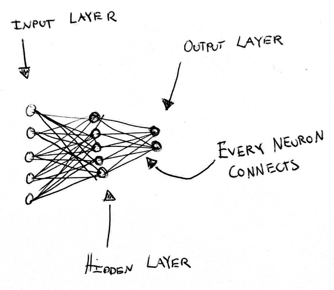
• Input layer. This is a representation of the data that we want to feed to the neural net. For example, the input layer for a 4x4 pixel grayscale image that looks like this could be [1, 1, 1, 0.2]. Meaning the first 3 pixels are darkest (1.0) and the last pixel is lighter (0.2).
• Hidden Layer. This is the layer that does a bunch of math on the input layer to convert it to our prediction. Training a model refers to changing the math of the hidden layer(s) to more often create an output like the training data. We will go into more detail with this layer in a moment. The values in the hidden layer are called weights.
• Output Layer. This layer will contain our final prediction. For example, if we feed it the rectangle from before we might want the output layer to be a single number to represent how “dark” a rectangle is, e.g.: 0.8.

For example for the image = [0.8, 0.7, 1, 1] we’d expect a value close to 1 (dark!).

In contrast, for = [0.2, 0.5, 0.4, 0.7] we expect something closer to 0 than to 1.

Let’s implement a neural network from our simple mental model. The goal of this neural network is to take a grayscale 2x2 image and tell us how “dark” it is where 0 is completely white , and 1 is completely black . We will initialize the hidden layer with some random values at first, in Python:

input_layer = [0.2, 0.5, 0.4, 0.7]
# We randomly initialize the weights (values) for the hidden layer... We will
# need to "train" to make these weights give us the output layers we desire. We
# will cover that shortly!
hidden_layer = [0.98, 0.4, 0.86, -0.08]

output_neuron = 0
# This is really matrix multiplication. We explicitly _do not_ use a
# matrix/tensor, because they add overhead to understanding what happens here
# unless you work with them every day--which you probably don't. More on using
# matrices later.
for index, input_neuron in enumerate(input_layer):
    output_neuron += input_neuron * hidden_layer[index]
print(output_neuron)
# => 0.68

Our neural network is giving us model() = 0.7 which is closer to ‘dark’ (1.0) than ‘light’ (0.0). When looking at this rectangle as a human, we judge it to be more bright than dark, so we were expecting something below 0.5!

The only real thing we can change in our neural network in its current form is the hidden layer’s values. How do we change the hidden layer values so that the output neuron is close to 1 when the rectangle is dark, and close to 0 when it’s light?

We could abandon this approach and just take the average of all the pixels. That would work well! However, that’s not really the point of a neural net… We’ll hit an impasse if we one day expand our model to try to implement recognize_letters_from_picture(img) or is_cat(img).

Fundamentally, a neural network is just a way to approximate any function. It’s really hard to sit down and write is_cat, but the same technique we’re using to implement average through a neural network can be used to implement is_cat. This is called the universal approximation theorem: an artificial neural network can approximate any function!

So, let’s try to teach our simple neural network to take the average() of the pixels instead of explicitly telling it that that’s what we want! The idea of this walkthrough example is to understand a neural net with very few values and low complexity, otherwise it’s difficult to develop an intuition when we move to 1,000s of values and 10s of layers, as real neural networks have.

We can observe that if we manually modify all the hidden layer attributes to 0.25, our neural network is actually an average function!

input_layer = [0.2, 0.5, 0.4, 0.7]
hidden_layer = [0.25, 0.25, 0.25, 0.25]

output_neuron = 0
for index, input_neuron in enumerate(input_layer):
    output_neuron += input_neuron * hidden_layer[index]

# Two simple ways of calculating the same thing!
#
# 0.2 * 0.25 + 0.5 * 0.25 + 0.4 * 0.25 + 0.7 * 25 = 0.45
print(output_neuron)
# Here, we divide by 4 to get the average instead of
# multiplying each element.
#
# (0.2 + 0.5 + 0.4 + 0.7) / 4 = 0.45
print(sum(input_layer) / 4)

model() = 0.45 sounds about right. The rectangle is a little lighter than it’s dark.

But that was cheating! We only showed that we can implement average() by simply changing the hidden layer’s values. But that won’t work if we try to implement something more complicated. Let’s go back to our original hidden layer initialized with random values:

hidden_layer = [0.98, 0.4, 0.86, -0.08]

How can we teach our neural network to implement average?

Training our Neural Network

To teach our model, we need to create some training data. We’ll create some rectangles and calculate their average:

rectangles = []
rectangle_average = []

for i in range(0, 1000):
    # Generate a 2x2 rectangle [0.1, 0.8, 0.6, 1.0]
    rectangle = [round(random.random(), 1),
                 round(random.random(), 1),
                 round(random.random(), 1),
                 round(random.random(), 1)]
    rectangles.append(rectangle)
    # Take the _actual_ average for our training dataset!
    rectangle_average.append(sum(rectangle) / 4)

Brilliant, so we can now feed these to our little neural network and get a result! Next step is for our neural network to adjust the values in the hidden layer based on how its output compares with the actual average in the training data. This is called our loss function: large loss, very wrong model; small loss, less wrong model. We can use a standard measure called mean squared error:

# Take the average of all the differences squared!
# This calculates how "wrong" our predictions are.
# This is called our "loss".
def mean_squared_error(actual, expected):
    error_sum = 0
    for a, b in zip(actual, expected):
        error_sum += (a - b) ** 2
    return error_sum / len(actual)

print(mean_squared_error([1.], [2.]))
# => 1.0
print(mean_squared_error([1.], [3.]))
# => 4.0

Now we can implement train():

def model(rectangle, hidden_layer):
    output_neuron = 0.
    for index, input_neuron in enumerate(rectangle):
        output_neuron += input_neuron * hidden_layer[index]
    return output_neuron

def train(rectangles, hidden_layer):
  outputs = []
  for rectangle in rectangles:
      output = model(rectangle, hidden_layer)
      outputs.append(output)
  return outputs

hidden_layer = [0.98, 0.4, 0.86, -0.08]
outputs = train(rectangles, hidden_layer)

print(outputs[0:10])
# [1.472, 0.7, 1.369, 0.8879, 1.392, 1.244, 0.644, 1.1179, 0.474, 1.54]
print(rectangle_average[0:10])
# [0.575, 0.45, 0.549, 0.35, 0.525, 0.475, 0.425, 0.65, 0.4, 0.575]
mean_squared_error(outputs, rectangle_average)
# 0.4218

A good mean squared error is close to 0. Our model isn’t very good. But! We’ve got the skeleton of a feedback loop in place for updating the hidden layer.

Updating the Hidden Layer with Gradient Descent

Now what we need is a way to update the hidden layer in response to the mean squared error / loss. We need to minimize the value of this function:

mean_squared_error(
  train(rectangles, hidden_layer),
  rectangle_average
)

As noted earlier, the only thing we can really change here are the weights in the hidden layer. How can we possibly know which weights will minimize this function?

We could randomize the weights, calculate the loss (how wrong the model is, in our case, with mean squared error), and then save the best ones we see after some period of time.

We could possibly speed this up. If we have good weights, we could try to add some random numbers to those. See if loss improves. This could work, but it sounds slow… and likely to get stuck in some local maxima and not give a very good result. And it’s trouble scaling this to 1,000s of weights…

Instead of embarking on this ad-hoc randomization mess, it turns out that there’s a method called gradient descent to minimize the value of a function! Gradient descent builds on a bit of calculus that you may not have touched on since high school. We won’t go into depth here, but try to introduce just enough that you understand the concept. ³

Let’s try to understand gradient descent. Consider some random function whose graph might look like this:

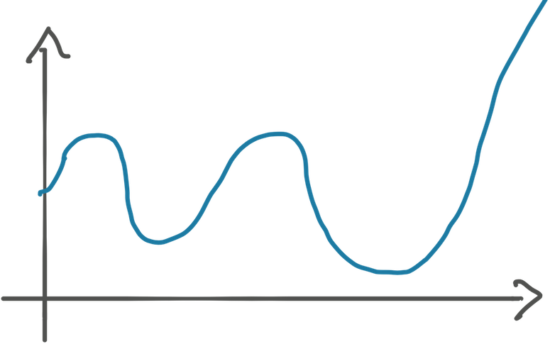
How do we write code to find the minimum, the deepest (second) valley, of this function?

Let’s say that we’re at x=1 and we know the slope of the function at this point. The slope is “how fast the function grows at this very point.” You may remember this as the derivative. The slope at x=1 might be -1.5. This means that every time we increase x += 1, it results in y -= 1.5. We’ll go into how you figure out the slope in a bit, let’s focus on the concept first.

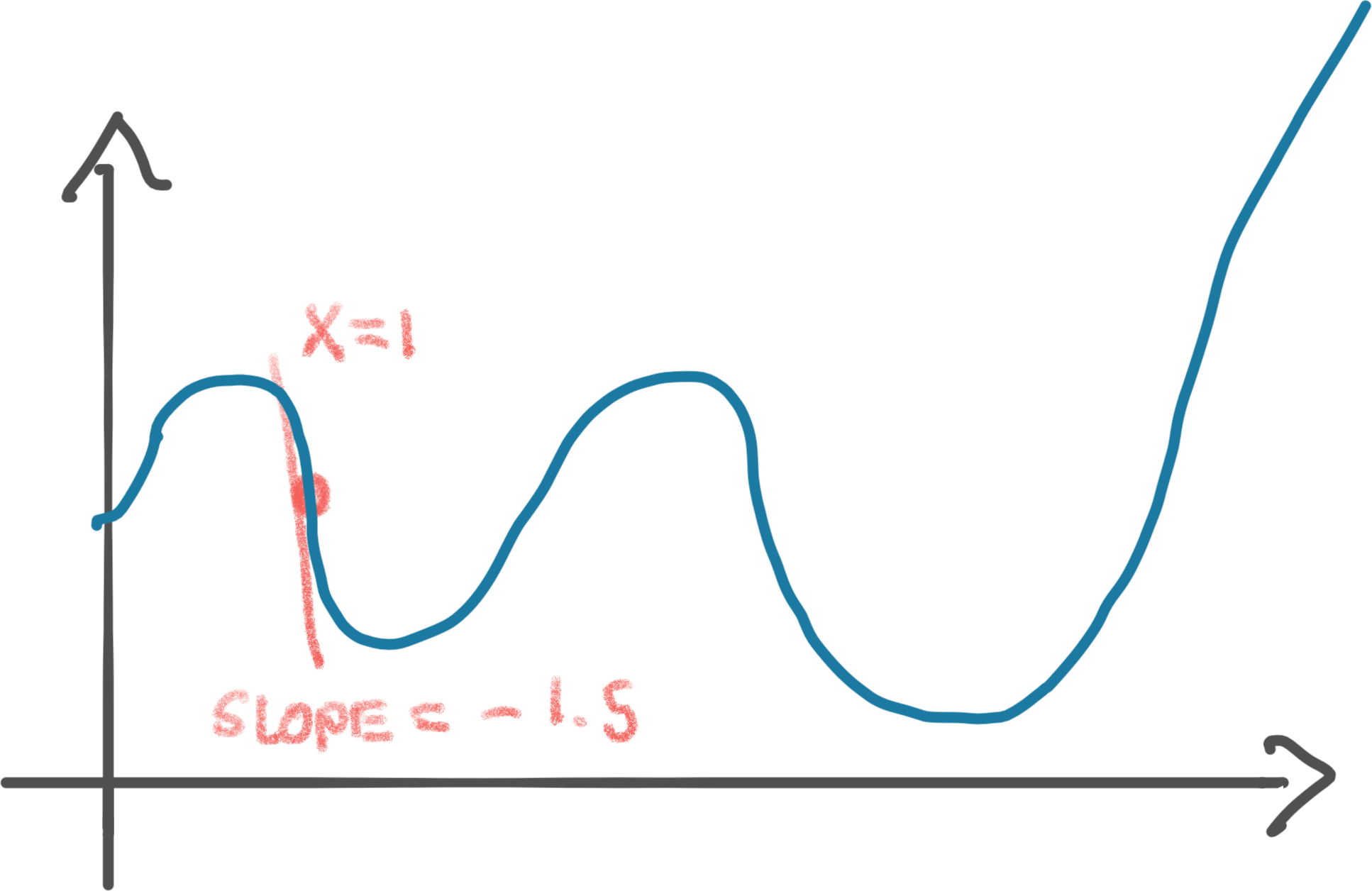
The idea of gradient descent is that since we know the value of our function, y, is decreasing as we increase x, we can increase x proportionally to the slope. In other words, if we increase x by the slope, we step towards the valley by 1.5.

Let’s take that step of x += 1.5:

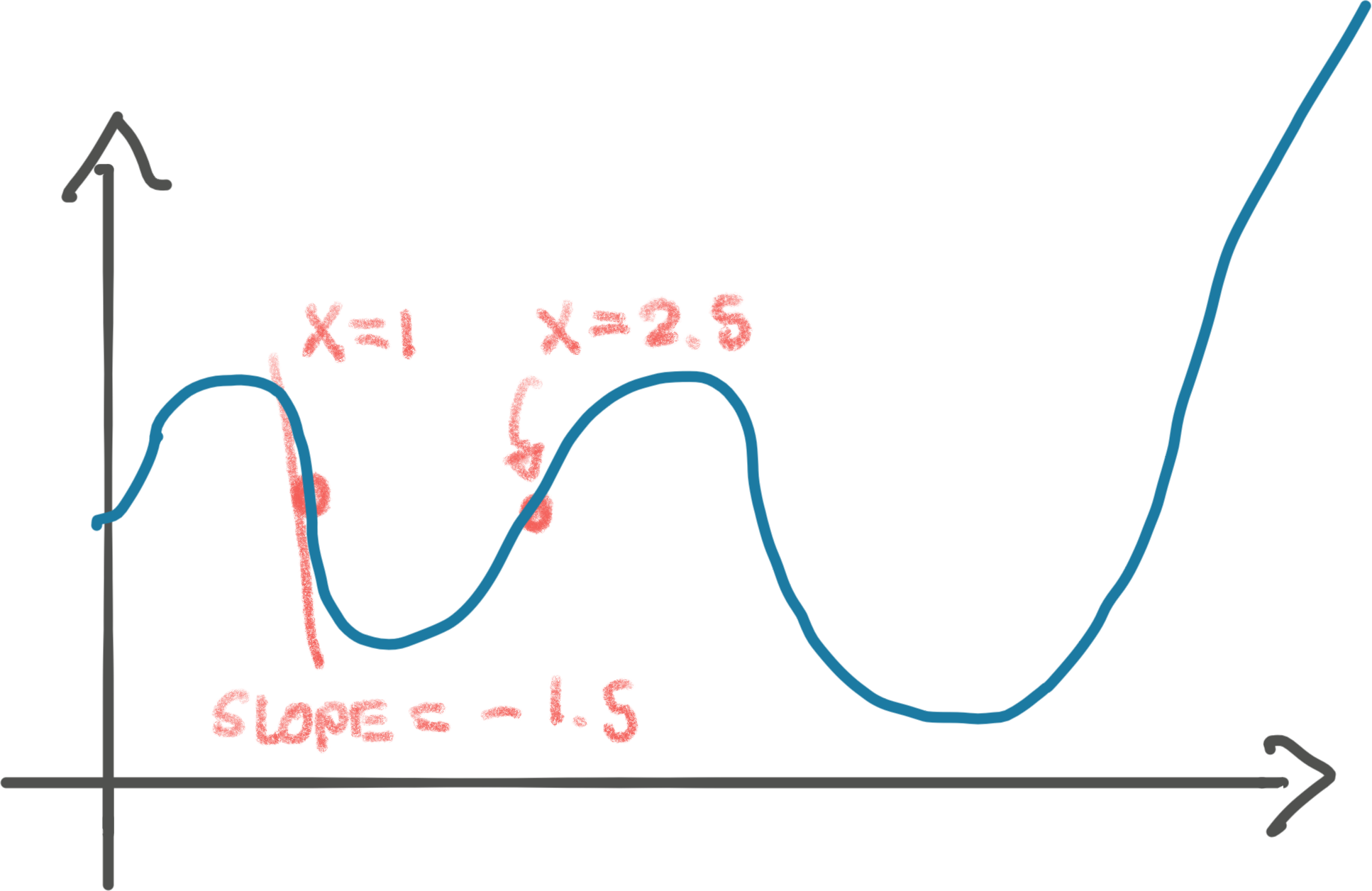
Ugh, turned out that we stepped too far, past this valley! If we repeat the step, we’ll land somewhere on the left side of the valley, to then bounce back on the right side. We might never land in the bottom of the valley. Bummer. Either way, this isn’t the global minimum of the function. We return to that in a moment!

We can fix the overstepping easily by taking smaller steps. Perhaps we should’ve stepped by just $0.1 * 1.5 = 0.15$ instead. That would’ve smoothly landed us at the bottom of the valley. That multiplier, 0.1, is called the learning rate in gradient descent.

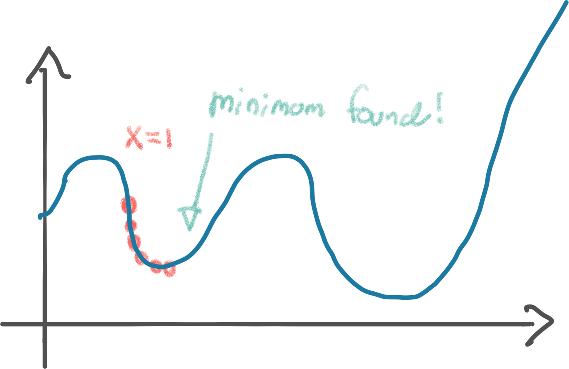
But hang on, that’s not actually the minimum of the function. See that valley to the right? That’s the actual global minimum. If our initial x value had been e.g. 3, we might have found the global minimum instead of our local minimum.

Finding the global minimum of a function is hard. Gradient descent will give us a minimum, but not the minimum. Unfortunately, it turns out it’s the best weapon we have at our disposal. Especially when we have big, complicated functions (like a neural net with millions of neurons). Gradient descent will not always find the global minimum, but something pretty good.

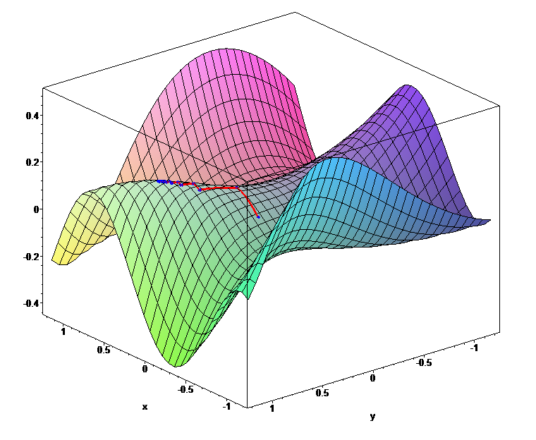
This method of using the slope/derivative generalizes. For example, consider optimizing a function in three-dimensions. We can visualize the gradient descent method here as rolling a ball to the lowest point. A big neural network is 1000s of dimensions, but gradient descent still works to minimize the loss!

Finalizing our Neural Network from scratch

Let’s summarize where we are:

• We can implement a simple neural net: model().
• Our neural net can figure out how wrong it is for a training set: loss(train()).
• We have a method, gradient descent, for tuning our hidden layer’s weights for the minimum loss. I.e. we have a method to adjust those four random values in our hidden layer to take a better average as we iterate through the training data.

Now, let’s implement gradient descent and see if we can make our neural net learn to take the average grayscale of our small rectangles:

def model(rectangle, hidden_layer):
    output_neuron = 0.
    for index, input_neuron in enumerate(rectangle):
        output_neuron += input_neuron * hidden_layer[index]
    return output_neuron

def train(rectangles, hidden_layer):
  outputs = []
  for rectangle in rectangles:
      output = model(rectangle, hidden_layer)
      outputs.append(output)

  mean_squared_error(outputs, rectangle_average)

  # We go through all the weights in the hidden layer. These correspond to all
  # the weights of the function we're trying to minimize the value of: our
  # model, respective of its loss (how wrong it is).
  # 
  # For each of the weights, we want to increase/decrease it based on the slope.
  # Exactly like we showed in the one-weight example above with just x. Now
  # we just have 4 values instead of 1! Big models have billions.
  for index, _ in enumerate(hidden_layer):
    learning_rate = 0.1
    # But... how do we get the slope/derivative?!
    hidden_layer[index] -= learning_rate * hidden_layer[index].slope

  return outputs

hidden_layer = [0.98, 0.4, 0.86, -0.08]
train(rectangles, hidden_layer)

Automagically computing the slope of a function with autograd

The missing piece here is to figure out the slope() after we’ve gone through our training set. Figuring out the slope/derivative at a certain point is tricky. It involves a fair bit of math. I am not going to go into the math of calculating derivatives. Instead, we’ll do what all the machine learning libraries do: automatically calculate it. ⁴

Minimizing the loss of a function is absolutely fundamental to machine learning. The functions (neural networks) are so complicated that manually sitting down to figure out the derivative like you might’ve done in high school is not feasible. It’s the mathematical equivalent of writing assembly to implement a website.

Let’s show one simple example of finding the derivative of a function, before we let the computers do it all for us. If we have $f(x) = x^2$, then you might remember from calculus classes that the derivative is $f'(x) = 2x$. In other words, $f(x)$’s slope at any point is 2x, telling us it’s increasing non-linearly. Well that’s exactly how we understand $x^2$, perfect! This means that for $x = 2$ the slope is $4$.

With the basics in order, we can use an autograd package to avoid the messy business of computing our own derivatives. autograd is an automatic differentiation engine. grad stands for gradient, which we can think of as the derivative/slope of a function with more than one parameter.

It’s best to show how it works by using our example from before:

import torch

# A tensor is a matrix in PyTorch. It is the fundamental data-structure of neural
# networks. Here we say PyTorch, please keep track of the gradient/derivative
# as I do all kinds of things to the parameter(s) of this tensor.
x = torch.tensor(2., requires_grad=True)

# At this point we're applying our function f(x) = x^2.
y = x ** 2

# This tells `autograd` to compute the derivative values for all the parameters
# involved. Backward is neural network jargon for this operation, which we'll
# explain momentarily.
y.backward()

# And show us the lovely gradient/derivative, which is 4! Sick.
print(x.grad)
# => 4

autograd is the closest to magic we get. I could do the most ridiculous stuff with this tensor, and it’ll keep track of all the math operations applied and have the ability to compute the derivative. We won’t go into how. Partly because I don’t know how, and this post is long enough.

Just to convince you of this, we can be a little cheeky and do a bunch of random stuff. I’m trying to really hammer this home, because this is what confused me the most when learning about neural networks. It wasn’t obvious to me that a neural network, including executing the loss function on the whole training set, is just a function, and however complicated, we can still take the derivative of it and use gradient descent. Even if it’s so many dimensions that it can’t be neatly visualized as a ball rolling down a hill.

autograd doesn’t complain as we add complexity and will still calculate the gradients. In this example we’ll even use a matrix/tensor with a few more elements and calculate an average (like our loss function mean_squared_error), which is the kind of thing we’ll calculate the gradients for in our neural network:

import random
import torch

x = torch.tensor([0.2, 0.3, 0.8, 0.1], requires_grad=True)
y = x

for _ in range(3):
    choice = random.randint(0, 2)
    if choice == 0:
        y = y ** random.randint(1, 10)
    elif choice == 1:
        y = y.sqrt()
    elif choice == 2:
        y = y.atanh()

y = y.mean()
# This walks "backwards" y all the way to the parameters to
# calculate the derivates / gradient! Pytorch keeps track of a graph of all the
# operations.
y.backward()

# And here are how quickly the function is changing with respect to these
# parameters for our randomized function.
print(x.grad)
# => tensor([0.0157, 0.0431, 0.6338, 0.0028])

Let’s use autograd for our neural net and then run it against our square from earlier model() = 0.45:

import torch as torch

def model(rectangle, hidden_layer):
    output_neuron = 0.
    for index, input_neuron in enumerate(rectangle):
        output_neuron += input_neuron * hidden_layer[index]
    return output_neuron

def train(rectangles, hidden_layer):
  outputs = []
  for rectangle in rectangles:
      output = model(rectangle, hidden_layer)
      outputs.append(output)

  # How wrong were we? Our 'loss.'
  error = mean_squared_error(outputs, rectangle_average)

  # Calculate the gradient (the derivate for all our weights!)
  # This walks "backwards" from the error all the way to the weights to
  # calculate them
  error.backward()

  # Now let's go update the weights in our hidden layer per our gradient.
  # This is what we discussed before: we want to find the valley of this
  # four-dimensional space/four-weight function. This is gradient descent!
  for index, _ in enumerate(hidden_layer):
    learning_rate = 0.1
    # hidden_layer.grad is something like [0.7070, 0.6009, 0.6840, 0.5302]
    hidden_layer.data[index] -= learning_rate * hidden_layer.grad.data[index]

  # We have to tell `autograd` that we've just finished an epoch to reset.
  # Otherwise it'd calculate the derivative from multiple epochs.
  hidden_layer.grad.zero_()
  return error

# We use tensors now, but we just use them as if they were normal lists.
# We only use them so we can get the gradients.
hidden_layer = torch.tensor([0.98, 0.4, 0.86, -0.08], requires_grad=True)

print(model([0.2,0.5,0.4,0.7], hidden_layer))
# => 0.6840000152587891

train(rectangles, hidden_layer)

# The hidden layer's weights are nudging closer to [0.25, 0.25, 0.25, 0.25]!
# They are now [ 0.9093,  0.3399,  0.7916, -0.1330]
print(f"After: {model([0.2,0.5,0.4,0.7], hidden_layer)}")
# => 0.5753424167633057
# The average of this rectangle is 0.45, closer... but not there yet

This blew my mind the first time I did this. Look at that. It’s optimizing the hidden layer for all weights in the right direction! We’re expecting them all to nudge towards $0.25$ to implement average(). We haven’t told it anything about average, we’ve just told it how wrong it is through the loss.

But, the hidden layer isn’t all $0.25$ quite yet, as we expect for it to implement average. So how do we get them to that? Well, let’s try to repeat the gradient descent process 100 times and see if we’re getting even better!

# An epoch is a training pass over the full data set!
for epoch in range(100):
   error = train(rectangles, hidden_layer)
   print(f"Epoch: {epoch}, Error: {error}, Layer: {hidden_layer.data}\n\n")
   # 
   #  Epoch: 99, Error: 0.0019292341312393546, Layer: tensor([0.3251, 0.2291, 0.3075, 0.1395])


print(model([0.2,0.5,0.4,0.7], hidden_layer).item())
# => 0.4002

Pretty close, but not quite there. I ran it for $300$ times (an iteration over the full training set is referred to as an epoch, so 300 epochs) instead, and then I got:

print(model([0.2,0.5,0.4,0.7], hidden_layer).item())
# Epoch: 299, Error: 1.8315197394258576e-06, Layer: tensor([0.2522, 0.2496, 0.2518, 0.2465])
# tensor(0.4485, grad_fn=<AddBackward0>)

Boom! Our neural net has almost learned to take the average, off by just a scanty $0.002$. If we fine-tuned the learning rate and number of epochs we could probably get it there, but I’m happy with this. model() = 0.448:

That’s it. That’s your first neural net:

OK, so you just implemented the most complicated average function I’ve ever seen…

Sure did. The thing is, that if we adjusted it for looking for cats, it’s the least complicated is_cat you’ll ever see. Because our neural network could implement that too by changing the training data. Remember, a neural network with enough neurons can approximate any function. You’ve just learned all the building blocks to do it. We just started with the simplest possible example.

If you give the hidden layer some more neurons, this neural net will be able to recognize handwritten numbers with decent accuracy (possible fun exercise for you, see bottom of article), like this one:

Activation Functions

To be truly powerful, there is one paramount modification we have to make to our neural net. Above, we were implementing the $average$ function. However, were our neural net to implement which_digit(png) or is_cat(jpg) then it wouldn’t work.

Recognizing handwritten digits isn’t a linear function, like average(). It’s non-linear. It’s a crazy function, with a crazy shape (unlike a linear function). To create crazy functions with crazy shapes, we have to introduce a non-linear component to our neural network. This is called an activation function. It can be e.g. $ReLu(x) = max(0, x)$. There are many kinds of activation functions that are good for different things. ⁵

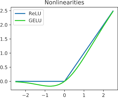
We can apply this simple operation to our neural net:

def model(rectangle, hidden_layer):
    output_neuron = 0.
    for index, input_neuron in enumerate(rectangle):
        output_neuron += input_neuron * hidden_layer[index]
    return max(0, output_neuron)

Now, we only have a single neuron/weight… that isn’t much. Good models have 100s, and the biggest models like GPT-3 have billions. So this won’t recognize many digits or cats, but you can easily add more weights!

Matrices

The core operation in our model, the for loop, is matrix multiplication. We could rewrite it to use them instead, e.g. rectangle @ hidden_layer. PyTorch will then do the exact same thing. Except, it’ll now execute in C-land. And if you have a GPU and pass some extra weights, it’ll execute on a GPU, which is even faster. When doing any kind of deep learning, you want to avoid writing any Python loops. They’re just too slow. If you ran the code above for the 300 epochs, you’ll see that it takes minutes to complete. I left matrices out of it to simplify the explanation as much as possible. There’s plenty going on without them.

Next steps to implement your own neural net from scratch

Even if you’ve carefully read through this article, you won’t fully grasp it yet until you’ve had your own hands on it. Here are some suggestions on where to go from here, if you’d like to move beyond the basic understanding you have now:

1. Get the notebook running and study the code
2. Change it to far larger rectangles, e.g. 100x100
3. Add biases in addition to the weights. A model doesn’t just have weights that are multiplied onto the inputs, but also biases that are added (+) onto the inputs in each layer.
4. Rewrite the model to use PyTorch tensors for matrix operations, as described in the previous section.
5. Add 1-2 more layers to the model. Try to have them have different sizes.
6. Change the tensors to run on GPU (see the PyTorch documentation) and see the performance speed up! Increase the size of the training set and rectangles to really be able to tell the difference. Make sure you change Runtime > Change Runtime Type in Collab to run on a GPU.
7. This is a difficult step that will likely take a while, but it’ll be well worth it: Adapt the code to recognize handwritten letters from the MNIST dataset dataset. You’ll need to use pillow to turn the pixels into a large 1-dimensional tensor as the input layer, as well as a non-linear activation function like Sigmoid or ReLU. Use Nielsen’s book as a reference if you get stuck, which does exactly this.

I thoroughly hope you enjoyed this walkthrough of a neural net from scratch! In a future issue we’ll use the mental model we’ve built up here to do some napkin math on expected performance on training and using neural nets.

Thanks to Vegard Stikbakke, Andrew Bugera and Jonathan Belotti for providing valuable feedback on drafts of this article.

You might also like...

• MySQL transactions per second vs fsyncs per second
• Using checksums to verify syncing 100M database records
• Shitlist Driven Development
• Increase HTTP Performance by Fitting In the Initial TCP Slow Start Window
• Inverted Index Performance and Merkle Tree Syncronization